How Kwai Scaled Multimodal Vector Search to 100 Billion Vectors on Apache Doris

TL;DR: Kwai runs multimodal vector search over 100 billion 2,048-dimensional embeddings, close to 1 PB of raw data, on Apache Doris, with filters and nearest-neighbor search in one SQL statement. Three design choices keep memory and scan cost down: IVF-ON-DISK holds only index metadata in memory, 4-bit RaBitQ compresses vectors 8x, and a global two-layer index limits each query to about 1% of the vectors. Compared with brute-force search, a query went from 42 minutes to 21 seconds.

At Kwai, the risk-control team segments users by comparing image embeddings. E-commerce search finds products from a photo, the ad team finds similar ad creatives, and model teams pull training data for large models. Each of these is a vector similarity search that usually also filters on structured business fields (scalar filters). A single use case can hold 100 billion 2,048-dimensional vectors, close to 1 PB of raw data.

Kwai now runs this workload on Apache Doris, where one SQL statement applies the scalar filters and the nearest-neighbor search together. On a production table of 100 billion vectors, a query that took 42 minutes with brute-force search now takes 21 seconds.

How does Kwai use Apache Doris today?

Kwai, the company behind the generative AI video tool Kling AI, already runs Apache Doris for several large workloads: a unified lakehouse that replaced ClickHouse and serves nearly 1 billion queries per day, trillion-scale ad analytics moved off ClickHouse and Elasticsearch, and company-wide A/B testing metrics that run up to 145x faster on a 2,000-node cluster.

Bleem, Kwai's heavily customized build of Apache Doris, supports core workloads such as advertising, A/B testing, risk-control user segmentation, and e-commerce data warehousing. It is one of the main platforms for big data analytics at Kwai, and vector search is its newest workload.

Why did Kwai need vector search at 100-billion scale?

As LLMs and AI agents went into production, the data engine team started getting two kinds of vector search requests:

Existing workloads that outgrew brute force. Risk-control user segmentation already ran similarity search on image embeddings by comparing each query with every row. That worked while the data was small. As data volumes grew sharply, the compute cost and latency became too high.
Analytics workloads that added vector search. Teams that had only analyzed structured data started using vectors for e-commerce semantic search and image-based product search, finding similar ad creatives, retrieving training data for large models, content moderation, and RAG-based agent applications.

Each 2,048-dimensional vector is about 8 KB, so a use case with 100 billion rows holds nearly 1 PB of raw vectors, which make up most of the storage cost. Quantized indexes are much smaller, and most queries return only the Top-K results. Those results go one of two ways:

Small Top-K (hundreds to thousands): returned to the client through an online API.
Large Top-K (millions to tens of millions): written to the data lake for downstream analysis or as training data for large models.

What did Kwai require from vector search?

These are batch and interactive analytics workloads, so the team defined success around recall (the share of the true nearest neighbors a search returns) and cost. Choosing a vector index at this scale means trading off recall, performance, and cost, and Kwai's rule was to hold recall at the target and make memory the first cost to cut.

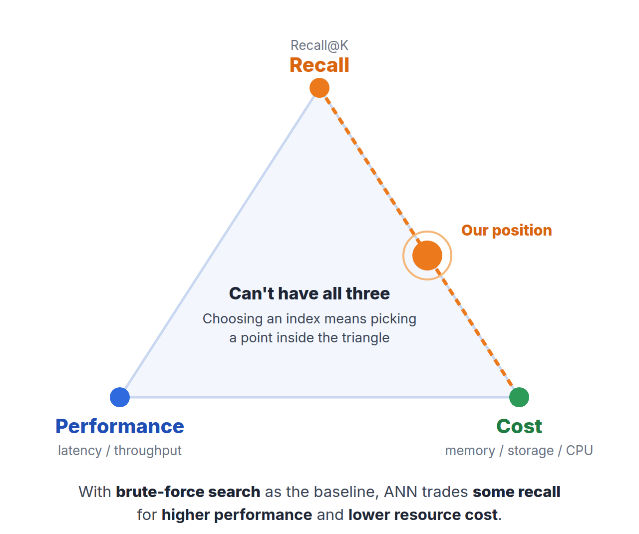
Figure 1. Choosing a vector index means picking a point inside the triangle of recall, performance, and cost. Kwai held recall at the target and pushed cost down.

The acceptance criteria:

Recall: meet a target recall rate, such as 95% or higher.
Cost: keep memory and compute cost as low as possible. With a 1 PB dataset, memory can't grow linearly with data size.
One database, correct results: a single SQL statement handles scalar filtering and nearest-neighbor search, every result satisfies the filters, and the query still returns enough rows when the filters match only a small fraction of the data.
Isolation: interactive queries (small K, low latency, higher concurrency), batch jobs (large K, high throughput), and ingestion share one platform without slowing each other down.
Large-K output: return hundreds of thousands to millions of neighbors, plus their raw vectors, without running out of memory.

Millisecond end-to-end latency, the goal in online search and recommendation, was out of scope.

The team chose to build on Doris, which as of version 4.1 supports structured queries, full-text search with inverted indexes and BM25 scoring, and vector search with HNSW, IVF, and IVF-ON-DISK indexes. These teams already used Doris, so Kwai could serve queries that combine all three in one system and reuse the scheduling, resource isolation, and monitoring it already had.

How does Kwai search 100 billion vectors on Apache Doris?

Memory cost: IVF-ON-DISK keeps only metadata in memory

Apache Doris builds its approximate nearest neighbor (ANN) indexes on the open-source Faiss library. HNSW, a graph-based index, gives high recall and low latency, but the whole index has to stay in memory. Standard IVF (inverted file index) groups vectors into clusters and stores each cluster as an inverted list, and it also keeps all of those lists in memory. At 100 billion vectors of about 8 KB each, the index is close to 1 PB, and keeping it in memory would take a cluster with hundreds of terabytes of RAM.

IVF-ON-DISK splits the index in two. The metadata (cluster centroids plus a slot table that records each inverted list's offset and length) is small and stays in memory. The inverted lists, by far the largest part, stay on disk. At query time, Doris compares the query vector with the centroids, picks the closest clusters (the nprobe parameter sets how many), and reads only those clusters' lists from disk. Those lists go into a dedicated ANN inverted-list cache, so hot lists stay in memory and cold lists load from local disk or remote storage on demand.

IVF-ON-DISK has the same recall as IVF-Flat (standard IVF with uncompressed vectors); moving the lists to disk adds I/O latency only for cold lists. Memory use no longer grows linearly with total data size.

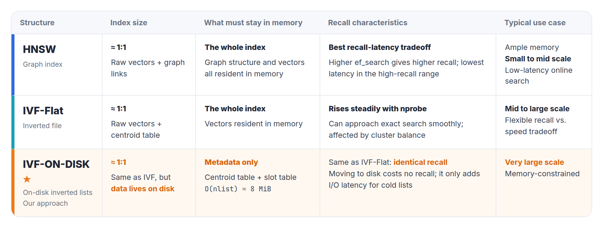
Figure 2. HNSW, IVF-Flat, and IVF-ON-DISK compared by index size, memory footprint, recall, and typical use.

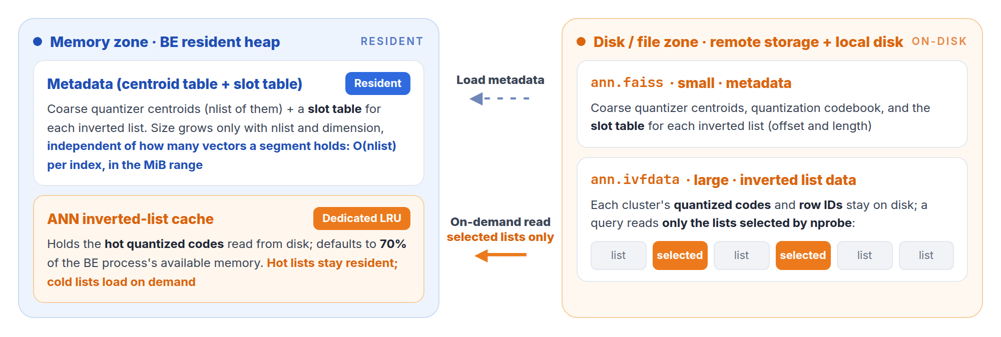
Figure 3. IVF-ON-DISK keeps the metadata in memory and reads only the inverted lists that nprobe selects.

Compression and recall: 4-bit RaBitQ quantization

With the index on disk, the next decision was how much to compress the vectors inside the inverted lists. Doris already supported scalar quantization (SQ) and product quantization (PQ), and the team added RaBitQ:

SQ is simple and loses little accuracy, but compression tops out at 4x to 8x.
PQ splits each vector into subvectors and clusters each subspace separately. It reaches very high compression ratios, but it loses some accuracy and needs a trained codebook that has to stay in memory.
RaBitQ needs no subspace split and no codebook. Its distance estimates come with a theoretical error bound, and that bound tightens as dimensionality rises, which suits Kwai's 2,048-dimensional embeddings.

Kwai chose 4-bit RaBitQ, which compresses vectors 8x. The results below compare its recall with PQ.

Scan cost: a global two-layer index on table partitions

By default, Doris builds a vector index for each data file (segment). At 100 billion rows, a single query touches so many segments that merging results across them and processing shard metadata become expensive.

The team moved IVF's clustering step up to the table level. They train global centroids on the full vector set, assign each vector to its nearest cluster, and use the cluster ID as the table's partition key. Each query then runs in two layers:

Layer 1 (partitions): during query planning, Doris compares the query vector with the global centroids and uses standard partition pruning to skip most partitions.
Layer 2 (segments): inside the few remaining partitions, Doris runs the segment-level IVF-ON-DISK + RaBitQ search.

High-dimensional embeddings tend to skew into a few giant clusters and many near-empty ones, which weakens partition pruning. To keep partitions evenly sized, the team trains centroids with a balanced K-Means algorithm that caps each cluster's size. With both layers, each query computes distances for about 1% of the table's vectors.

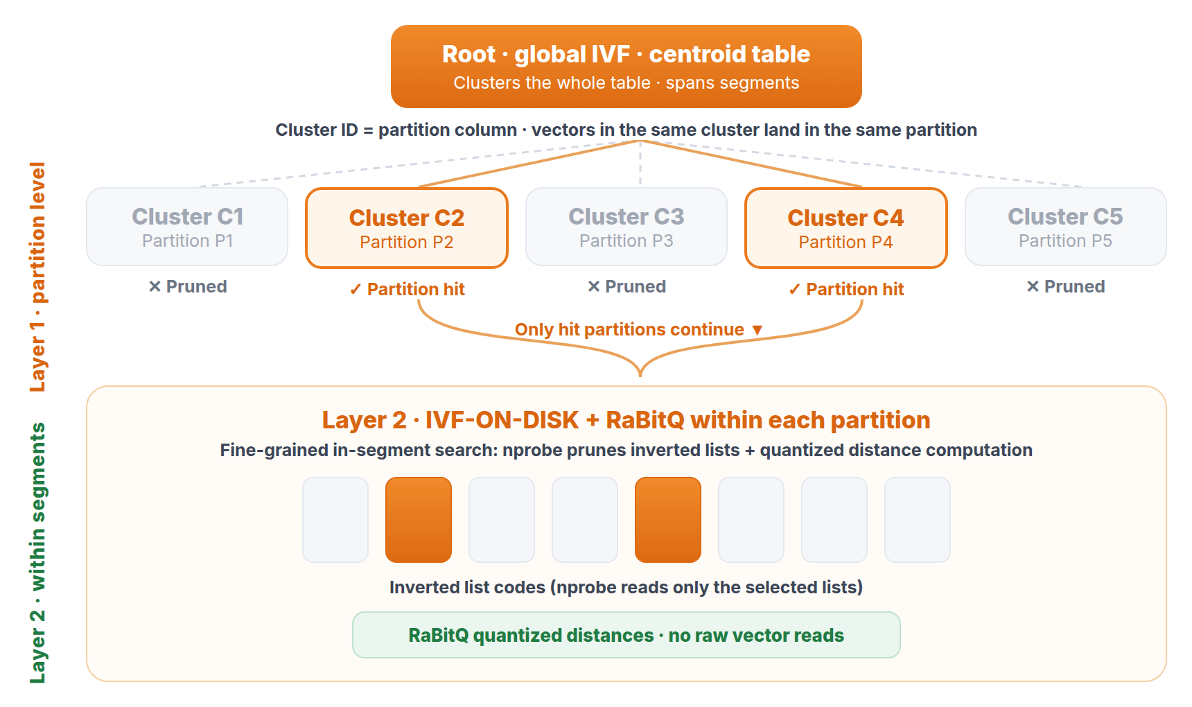
Figure 4. The global two-layer index: partition pruning on global centroids, then IVF-ON-DISK + RaBitQ inside the partitions that remain.

Correct filtered results: pre-filtering with a faster fallback

Every vector query uses pre-filtering: Doris applies the filters before the vector search. It first uses the inverted index to find the rows that match the filter conditions and collects their row IDs into an allowlist. The vector index then computes distances only for rows on that list, so every result satisfies the filters.

Doris handles two edge cases with a fallback: a filter the inverted index can't evaluate, and a candidate set so small that the vector index might return too few rows. In both cases, it switches to brute-force search over the candidate rows. A standard fallback reads the full floating-point vectors from disk and computes exact distances. Kwai's version looks up the RaBitQ codes already stored in each segment by row ID and estimates distances from them, switching between point reads and batch reads depending on what share of rows passed the filter.

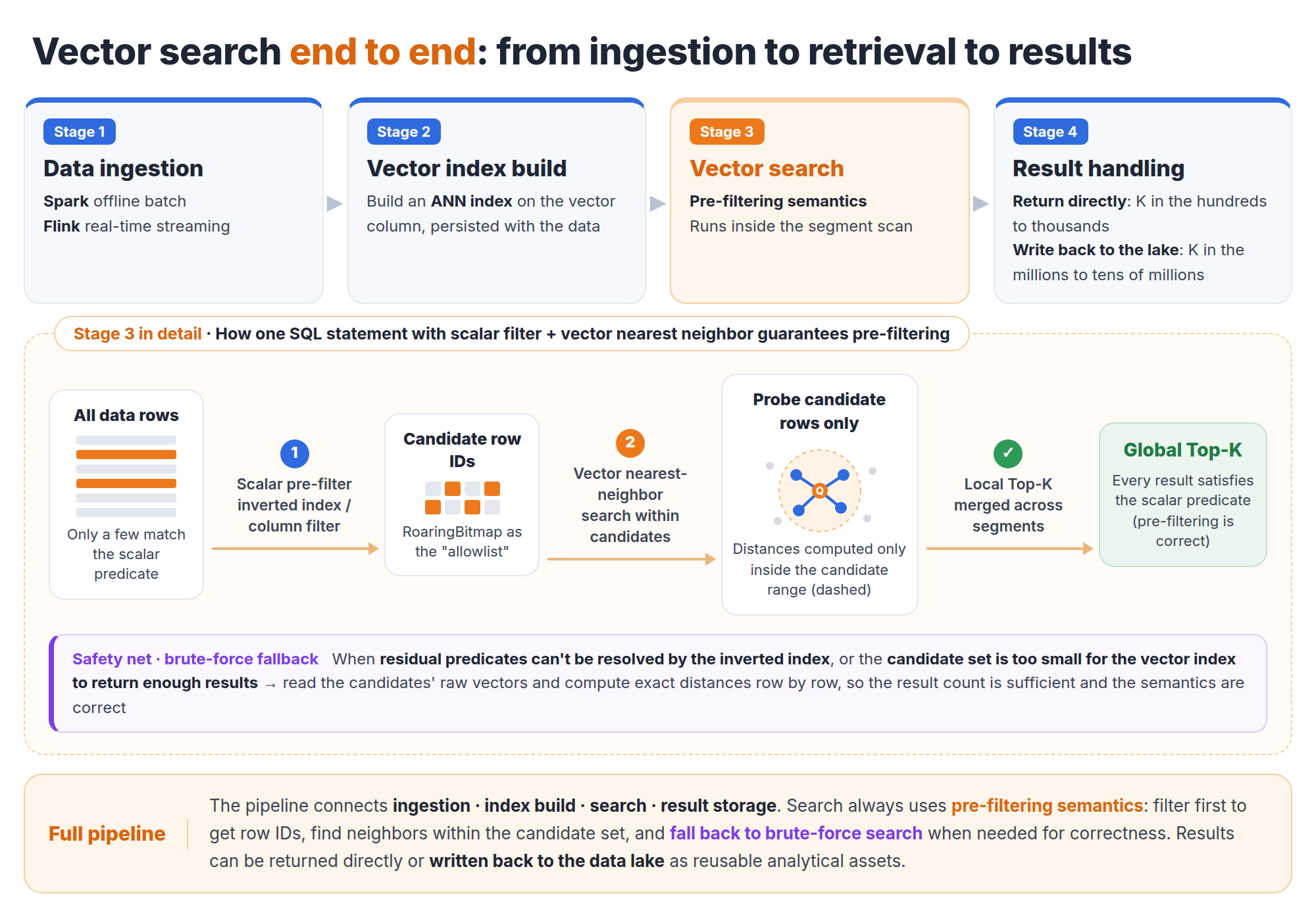
Figure 5. The end-to-end pipeline, with pre-filtering and the fallback shown in the search stage.

Isolation: compute groups and dedicated cache tiers

The deployment separates storage and compute. Compute nodes are divided into compute groups that share one copy of the data in remote storage:

Ingestion stays in its own group. Spark batch loads, Flink streaming writes, index builds, and background compaction all run in a dedicated ingestion compute group, so they don't take CPU or I/O from the query groups.
Indexes are warmed up before the first query. When the ingestion group finishes building a vector index, it tells the target query nodes to pull the index files to local disk. Consistent hashing routes each shard to a fixed node, so the node that was warmed up is the node that runs the query.
Vector indexes get their own caches. In memory, scalar columns use the general Page Cache and vector indexes use the ANN inverted-list cache, each with its own quota. On local disk, index files get a dedicated Index queue in the File Cache (the local disk cache). Reads check memory first, then local disk, and only a small amount of cold data has to come from remote storage.
Interactive and batch work get different settings. Each use case gets its own compute group and tunes search parameters such as nprobe through session variables. Interactive groups use short timeouts and fail fast, and batch groups get longer timeouts that favor throughput.

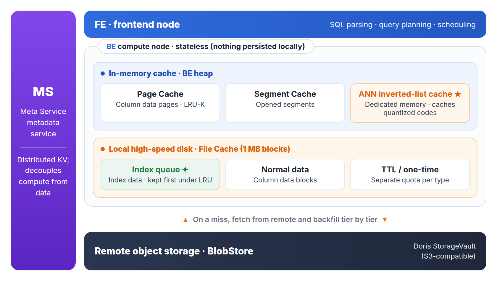
Figure 6. Cache tiers with storage and compute separated: in-memory caches on each backend (BE) node, File Cache queues on local disk, and remote object storage.

Large-K output: a SQL rewrite that separates sorting from vector fetches

Building a training dataset can mean pulling hundreds of thousands to millions of neighbors in one query, plus their raw vectors. Run as is, that query carries every 8 KB vector through the sort to a single node, which can easily run out of memory.

The team rewrote the query in plain SQL, with no changes to Doris itself. A subquery returns only primary keys and distances. After the global merge, the Top-K keys go to every node as a broadcast runtime filter, and each node reads the matching raw vectors locally, in parallel.

-- Rewritten large-K query (q is the query vector, K = 500,000)
SELECT t1.id, t1.embedding, t2.distance
FROM tbl t1 JOIN (
  SELECT id, l2_distance_approximate(embedding, q) AS distance
  FROM tbl ORDER BY distance LIMIT 500000
) t2 ON t1.id = t2.id;  -- t2 (id, distance) is broadcast to every node

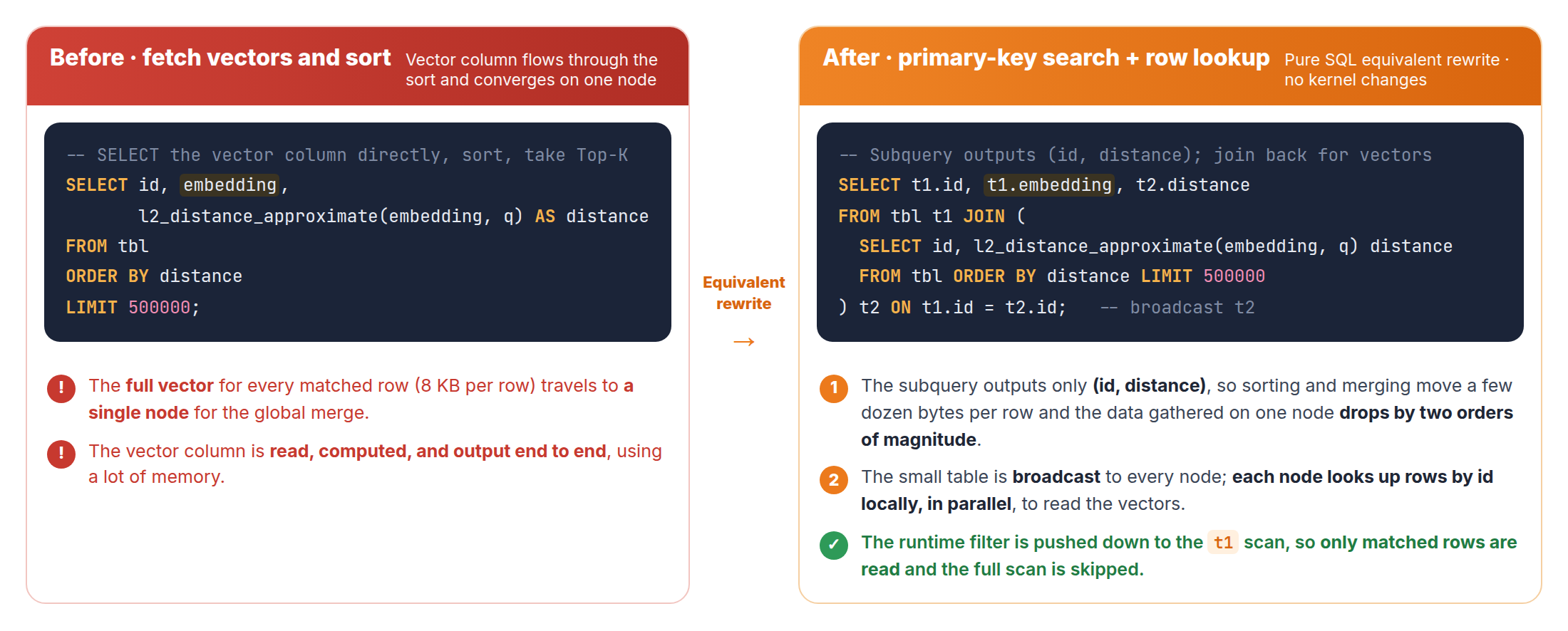
Figure 7. The equivalent SQL rewrite: the subquery returns only (id, distance), and a broadcast join fetches the vectors afterward.

Settings that mattered at this scale

Ingestion side: cap index build concurrency on each node, size segments so their row counts are in line with the number of clusters, enable asynchronous warm-up, and warm up only the vector index files.
Query side: tune nprobe for both layers per use case, enlarge the ANN inverted-list cache, turn off the general Page Cache for column data on very large datasets, and raise the fallback threshold so the inverted index handles as many filters as possible.

How much faster is the two-layer index than brute-force search?

100 billion vectors in production

The team tested the full design on a Kwai production table with 100 billion 2,048-dimensional vectors:

Layer 1: 1,024 global clusters, with each query probing the nearest 128 partitions.
Layer 2: IVF-ON-DISK + 4-bit RaBitQ inside each partition, probing 128 inverted lists.

Compared with brute-force search, the two-layer index made the query 120x faster (from 42 minutes to 21 seconds), scanned 4,800x less data, and used 57x less CPU time and 23x less peak memory.

Metric	Brute-force exact search	Layer 2 only (no partition pruning)	Two-layer index	Reduction
Query time	42.3 min	2.6 min	21 s	120x
Rows scanned	109.38 billion	14.98 billion	2.11 billion	51.8x
Bytes scanned	0.90 PB	1.34 TB	187.9 GB	4,805x
CPU time	800 h	106 h	13.9 h	57.5x
Peak memory	39.5 GB	1.99 GB	1.73 GB	22.9x

Table 1. Brute-force search, layer-2 ANN only, and the full two-layer index on Kwai's 100-billion-vector, 2,048-dimensional production table. Source: Kwai production test.

The middle column shows what the partition layer adds: with layer 2 alone, the same query still takes 2.6 minutes and scans 1.34 TB.

Recall at high dimensions: RaBitQ vs. PQ

To compare quantization methods at low and high dimensions, the team tested them on the public SIFT-1M benchmark (128 dimensions) and on KWAI-1M, a Kwai production dataset (2,048 dimensions).

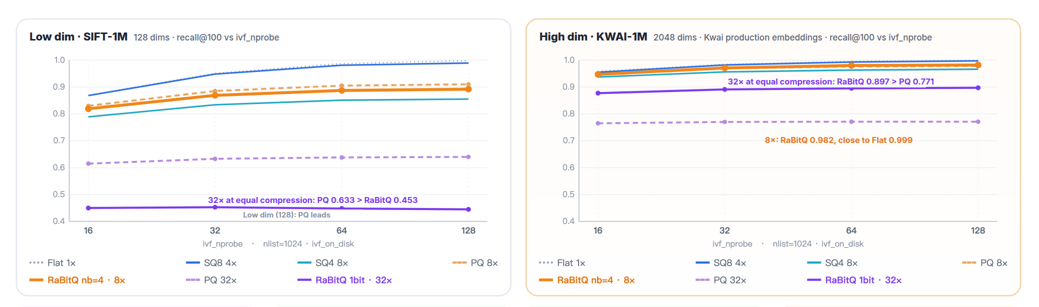
Figure 8. Recall@100 against ivf_nprobe on SIFT-1M (128 dimensions) and KWAI-1M (2,048 dimensions).

At 128 dimensions and the same 32x compression, PQ leads (0.633 recall@100 vs. 0.453 for 1-bit RaBitQ). At 2,048 dimensions the order reverses: 1-bit RaBitQ reaches 0.897 vs. 0.771 for PQ. The 4-bit RaBitQ setting Kwai chose reaches 0.982 recall@100 at 8x compression, close to the 0.999 of uncompressed (Flat) search and above the 95% recall target.

These recall figures come from the 1-million-vector datasets. The 100-billion-vector production test above measured speed and resource use.

Engineering improvements

Faster fallback: estimating distances from RaBitQ codes made the fallback 6.8x to 14x faster with 4x to 7x lower peak memory, and the estimates have a mean relative error of 0.1% against exact distances.
Large-K queries: with K in the millions, the SQL rewrite scanned about 15x less data and cut peak memory from 39 GB to 821 MB (about 47x lower), which removes the risk of out-of-memory (OOM) failures on these queries.
Balanced partitions: the size-capped K-Means cut the coefficient of variation of cluster sizes from 0.53 to 0.15. The largest partition went from 12x the size of the smallest to 2.3x.

Scorecard

Acceptance criterion	Result
Recall at or above target (95%+)	0.982 recall@100 with 4-bit RaBitQ on KWAI-1M (Flat: 0.999)
Low memory and compute cost	Compared with brute force: 23x lower peak memory, 57x less CPU time, 4,800x less data scanned; query time from 42 min to 21 s
Correct filtered results in one SQL statement	Pre-filtering on a row ID allowlist; fallback 6.8x to 14x faster with 0.1% mean relative error
Isolation between ingestion, interactive, and batch work	Separate ingestion and query compute groups, dedicated caches, and per-use-case timeouts (design; no benchmark reported)
Large-K output without running out of memory	Peak memory from 39 GB to 821 MB with K in the millions

When is this design the right fit?

The design fits batch and interactive analytics over very large embedding tables, where recall targets and memory cost matter more than millisecond latency. Four caveats apply:

Millisecond serving was out of scope. Cold inverted lists add disk I/O latency, and this post has no numbers for online search or recommendation.
HNSW still fits smaller, latency-critical workloads. When the index fits in memory, HNSW gives the best recall-latency tradeoff.
RaBitQ's edge depends on dimensionality. At the same 32x compression, PQ beat 1-bit RaBitQ at 128 dimensions; RaBitQ pulled ahead at 2,048.
Some pieces are Kwai's own work. Apache Doris 4.1 ships IVF and IVF_ON_DISK indexes with INT8, INT4, and PQ quantization. RaBitQ, the global two-layer index, and the RaBitQ-based fallback run in Bleem, and Kwai plans to contribute them upstream.

What's next for vector search at Kwai?

With vector search now running reliably at 100-billion scale, Kwai is working with the Doris community and plans to contribute this work upstream. The team's next steps:

Multimodal hybrid search and reranking: search text, image, and video vectors together with scalar signals, using multi-channel retrieval, result fusion, and reranking to catch results that any single channel would miss.
Decoupled vector storage: move fixed-length, read-only vector data out of regular columnar storage into separate binary files, with the main table keeping only logical pointers to them. Compaction then no longer has to decode, re-encode, read, and rewrite the vectors.
Multimodal search on the data lake: improve index pushdown for lake tables such as Apache Paimon, so Doris can use full-text and vector indexes on lake data directly and search it in place, without moving it.

Frequently asked questions

How do you run vector search on 100 billion vectors?

Keep most of the index on disk and read as little of it as possible per query. Kwai uses IVF-ON-DISK, which holds only cluster centroids and list offsets in memory, plus 4-bit RaBitQ to compress vectors 8x. A global two-layer index skips most partitions, so each query computes distances for about 1% of the vectors and finishes in 21 seconds instead of 42 minutes.

HNSW vs. IVF: which index works at 100-billion scale?

HNSW gives high recall and low latency, but its whole index must stay in memory, and standard IVF keeps its inverted lists in memory too. At 100 billion 2,048-dimensional vectors, that index is close to 1 PB. IVF-ON-DISK keeps only metadata in memory with the same recall as IVF-Flat, while HNSW still suits small to mid-scale, low-latency search.

Is RaBitQ better than product quantization (PQ)?

It depends on dimensionality. At 128 dimensions and 32x compression, PQ scored 0.633 recall@100 vs. 0.453 for 1-bit RaBitQ; at 2,048 dimensions, 1-bit RaBitQ scored 0.897 vs. 0.771 for PQ. The 4-bit RaBitQ setting Kwai uses reached 0.982 at 8x compression, and RaBitQ needs no trained codebook.

How does filtered vector search work in Apache Doris?

Doris uses pre-filtering: the inverted index finds the rows that match the filters, and the vector index computes distances only for those rows, so every result satisfies the filters. When a filter can't use the inverted index, or too few rows pass it, Doris falls back to brute-force search. Kwai's RaBitQ-based fallback is 6.8x to 14x faster than the standard one.

Is IVF-ON-DISK available in open-source Apache Doris?

Yes. Apache Doris 4.1 added IVF and IVF_ON_DISK vector indexes ("index_type" = "ivf_on_disk") plus INT8, INT4, and PQ quantization; see the IVF On-Disk docs. RaBitQ and the global two-layer index are Kwai's additions, which Kwai plans to contribute upstream. For the design behind Doris vector search, see How We Built Production Vector Search in Apache Doris.