






Kwai, developer of the popular generative AI video tool Kling AI, migrated its company-wide A/B testing metrics pipeline from Spark to Apache Doris. The rebuild made metrics computation up to 145x faster and cut resource consumption by 72% on a 2,000-node cluster with 100,000 compute units (CUs).
We have covered Kwai's Apache Doris adoption twice before, both times in the real-time serving layer for advertising workloads: first replacing ClickHouse with a unified lakehouse serving nearly 1 billion queries per day, then replacing Elasticsearch.
This time the story comes from a different team and a different workload: scheduled batch computation. Kwai's data platform department runs the company-wide A/B testing platform. Every Kwai business line depends on it for experiment metrics. At Kwai, every strategy change has to produce positive A/B test results before it reaches production.
Kwai previously ran the A/B testing platform on Spark, which had two challenges. The first was job runtime: a single execution path took about 21 minutes to compute, and a product team that wanted experiment results in the afternoon typically waited until the next morning, which pushed every decision back a day. The second was cost. As A/B experiment volume grew, compute cost on full-traffic experiments rose linearly with it.
Given the scale of the data, the Kwai data platform team treated the move from Spark to Apache Doris as a rebuild of the computation system. The team reworked the storage layout, distinct aggregation, user-defined function (UDF) execution, task scheduling, and frontend (FE) metadata management.
The results of the rebuild:
-
145x faster on a single execution path in A/B metrics production: 21 minutes down to 8.7 seconds.
-
30x faster on the longest execution path: 65 minutes down to 2.12 minutes.
-
72% lower resource consumption.
-
The largest single Apache Doris cluster running in production, at 2,000 backend (BE) nodes, 100,000 CUs, and a memory pool of several hundred terabytes.
-
FE recovery window cut from ~27 minutes to ~10 minutes, with metadata memory down from 4.16GB to 1.49GB.
How A/B metrics get computed
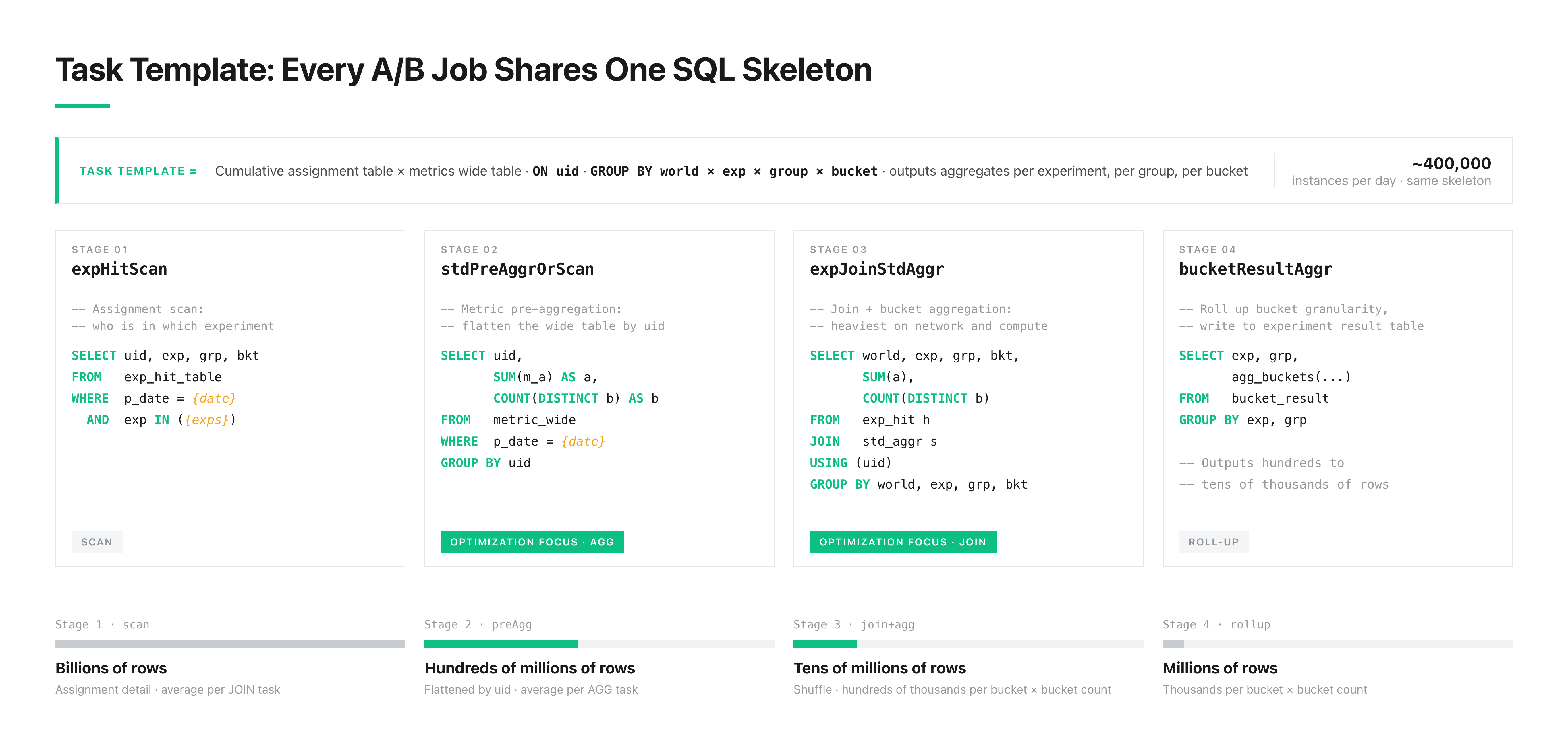
The A/B metrics pipeline has a stable structure. Input is fixed at two tables. The cumulative assignment table records which experiment and which group each user landed in. The metrics wide table records user behavior. Output is equally fixed: results aggregate by experiment, group, and bucket, and the result set usually runs from a few hundred to tens of thousands of rows.
The full computation takes four steps:
-
Scan the cumulative assignment table, filtering assignment records by date and experiment name.
-
Scan the metrics wide table, pre-aggregating by user ID (UID) and applying metric definitions.
-
Join the two tables on UID and aggregate at bucket granularity.
-
Roll up the bucket-level results and write them to the experiment result table.
Most of the cost sits in steps 2 and 3, which carry the join, the group-by aggregation, the network transfer, and the CPU cost all at once.
The defining characteristic of this workload: the join key is always UID, and the aggregation dimensions stay stable. The team could optimize aggressively because the query pattern was known in advance: one computation template, one execution path.
Why Apache Doris fits this workload
Most of the performance improvement came from aligning the workload's computation model with Doris's execution mechanism.
Apache Doris also brings three architectural advantages over Spark:
1. Pipeline execution reduces idle CPU threads
When Spark shuffles between two stages, data usually spills to disk, and downstream stages wait for all upstream work to finish, so threads tend to block. Apache Doris uses a pipeline model. A thread waiting on data yields to another task, which cuts CPU spin.
2. Vectorized execution improves batch efficiency
Spark SQL processes data row by row through its InternalRow format. Apache Doris uses columnar Blocks end to end, processing 4,096 rows per batch. A columnar layout suits single instruction multiple data (SIMD) batch processing on the CPU, and function call overhead amortizes from once per row to once per batch.
3. C++ runtime removes JVM overhead
Spark runs on the Java virtual machine (JVM), where garbage collection (GC) stop-the-world pauses and just-in-time (JIT) compilation warm-up both cost time. Apache Doris executes compiled C++ machine code with no JVM GC, reaching high execution efficiency immediately after startup.
Key optimizations: storage, compute, and scheduling
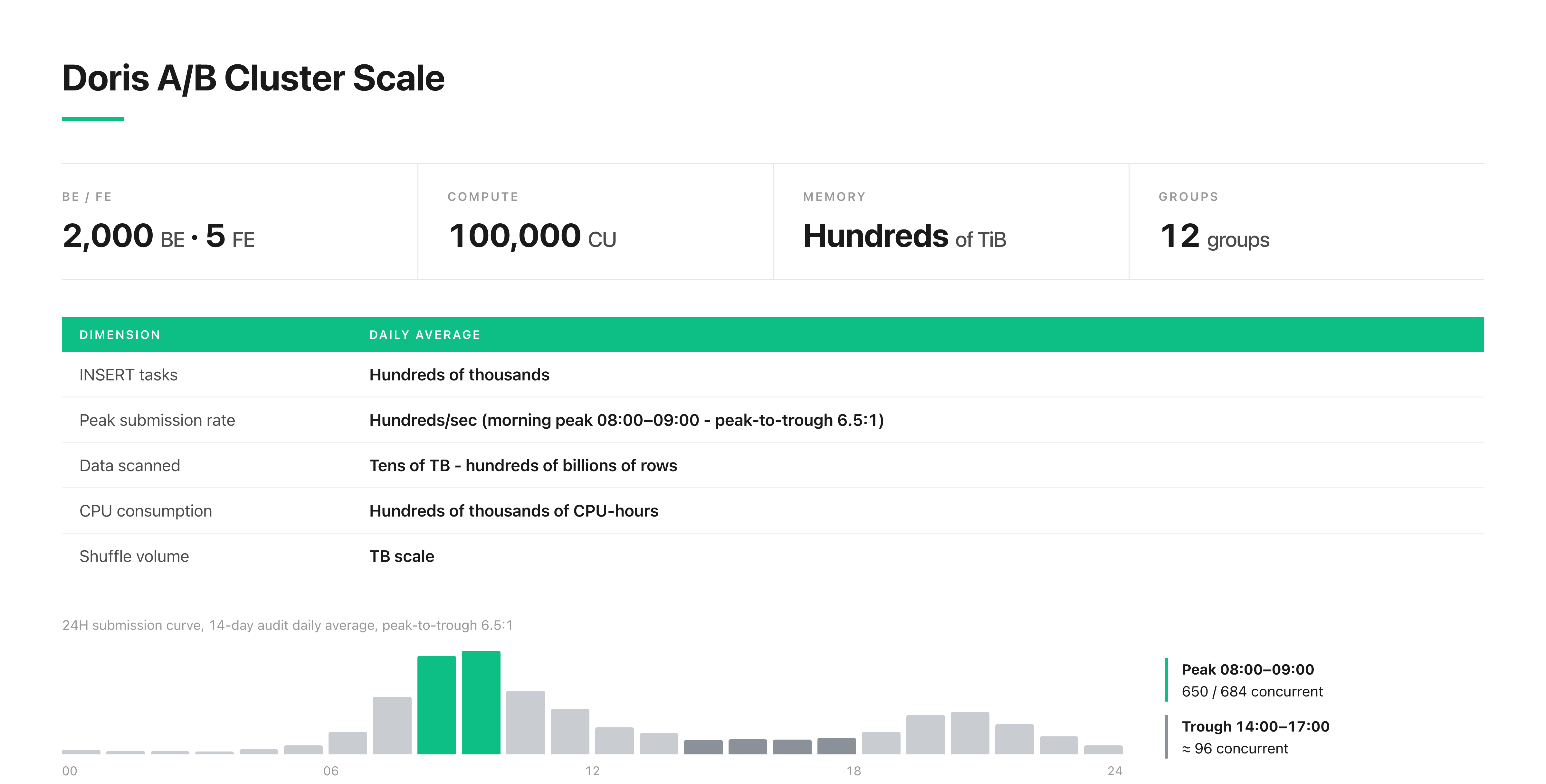
Doris's engine covered part of the gain. The rest came from shaping storage, computation, and scheduling around the A/B metrics template. The Doris A/B testing cluster runs 5 FE nodes, 2,000 BE nodes, 100,000 CUs, and a memory pool of several hundred terabytes, divided into 12 logical compute groups. A 14-day audit counted millions of tasks, with daily volume in the hundreds of thousands. Those tasks scan 40TB and hundreds of billions of rows a day.
At this size, a single inefficient operator multiplies its cost across every task on the cluster. After completing the engine migration, the team went further and optimized systematically across four layers: storage distribution, compute operators, low-level execution, and scheduling governance, all shaped around the characteristics of the A/B metrics template. A fifth area, FE metadata governance, became its own workstream once query performance stabilized.
Storage: eliminating cross-node shuffle with Colocate Join
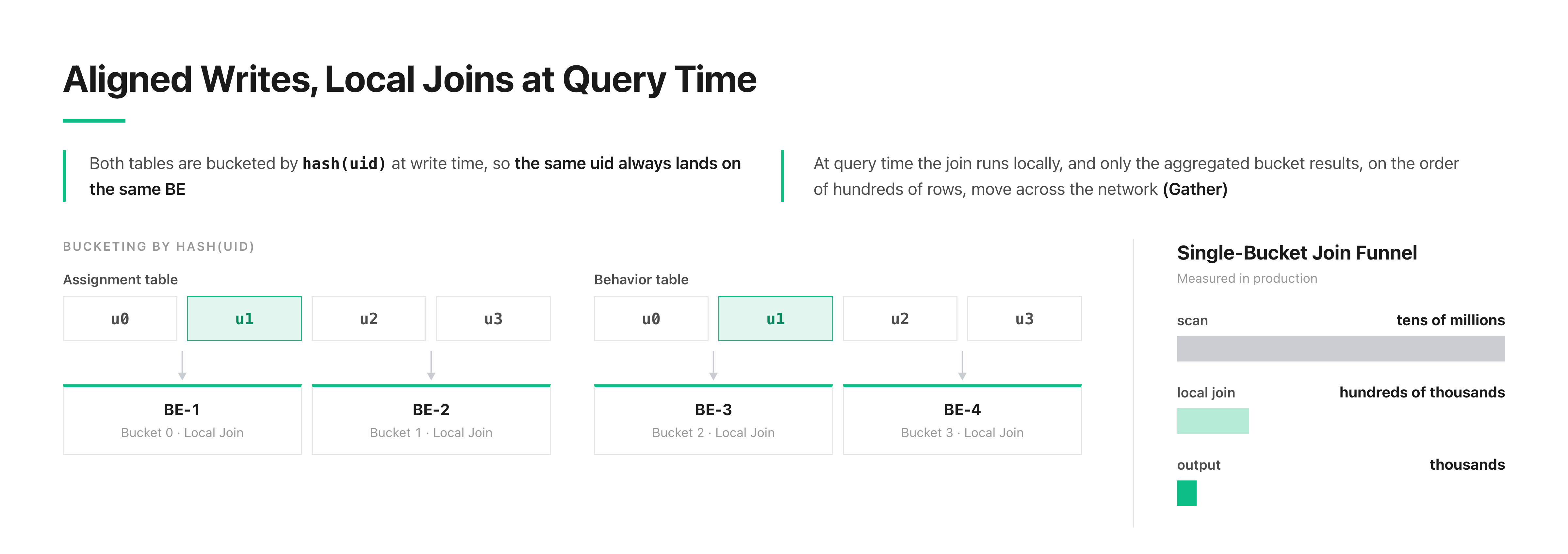
The first core optimization, Colocate Join, builds directly on the workload's fixed UID join key. The idea is to hash-bucket data by UID at write time, so rows sharing a UID always land on the same machine and in the same bucket.
At query time, the assignment table and the behavior table can then join locally, with no cross-node shuffle and no bulk data movement. Each node handles only the data in its local buckets, completes local aggregation, and contributes a small set of bucket-level results to the final merge.
Production numbers show the effect. A single bucket scans tens of millions of rows. The local join drops roughly 95% of them, leaving a few hundred thousand matched rows, and aggregation reduces that to a few thousand. Most of the data is filtered out inside the local node, and only the small post-join, post-aggregation result set travels over the network.
Two requirements matter when implementing Colocate Join:
-
Tables have to be hash-bucketed on the join key, which here is UID.
-
The two joined tables have to use exactly the same bucket count.
After adjusting the table structure, the team confirmed the execution plan with EXPLAIN. The optimization is only active when the plan shows Colocated. A plan that still contains Shuffle usually means the bucket counts, distribution keys, or Colocate configuration on the two tables are misaligned.
Compute: Local Distinct Grouping Sets
Colocate Join removed the cross-node shuffle from the join. In the compute layer, deduplication operators could still introduce a new global shuffle.
A/B metrics SQL uses Grouping Sets heavily, because a single query has to emit aggregates for several dimension combinations at once. In Doris's native execution framework, the standard two-phase optimization for Distinct did not cover the Grouping Sets + Distinct combination, so those queries still triggered a global shuffle, with high network cost and peak memory pressure.
The team designed and implemented a Local Distinct Grouping Sets rewrite for this. Colocate bucketing already guarantees that rows sharing a UID sit together locally, so deduplication can run locally on each compute node. Each node completes a local Distinct first, then the local results go through a global aggregation, which lowers shuffle cost while preserving semantics.
The optimization offers two modes:
-
Transparent rewrite: the optimizer recognizes the Grouping Sets + Distinct pattern and rewrites it to the local computation path, with no change to business SQL.
-
Explicit invocation: teams can specify local deduplication directly with Distinct Local syntax, for cases the optimizer does not cover but that the team has confirmed safe.
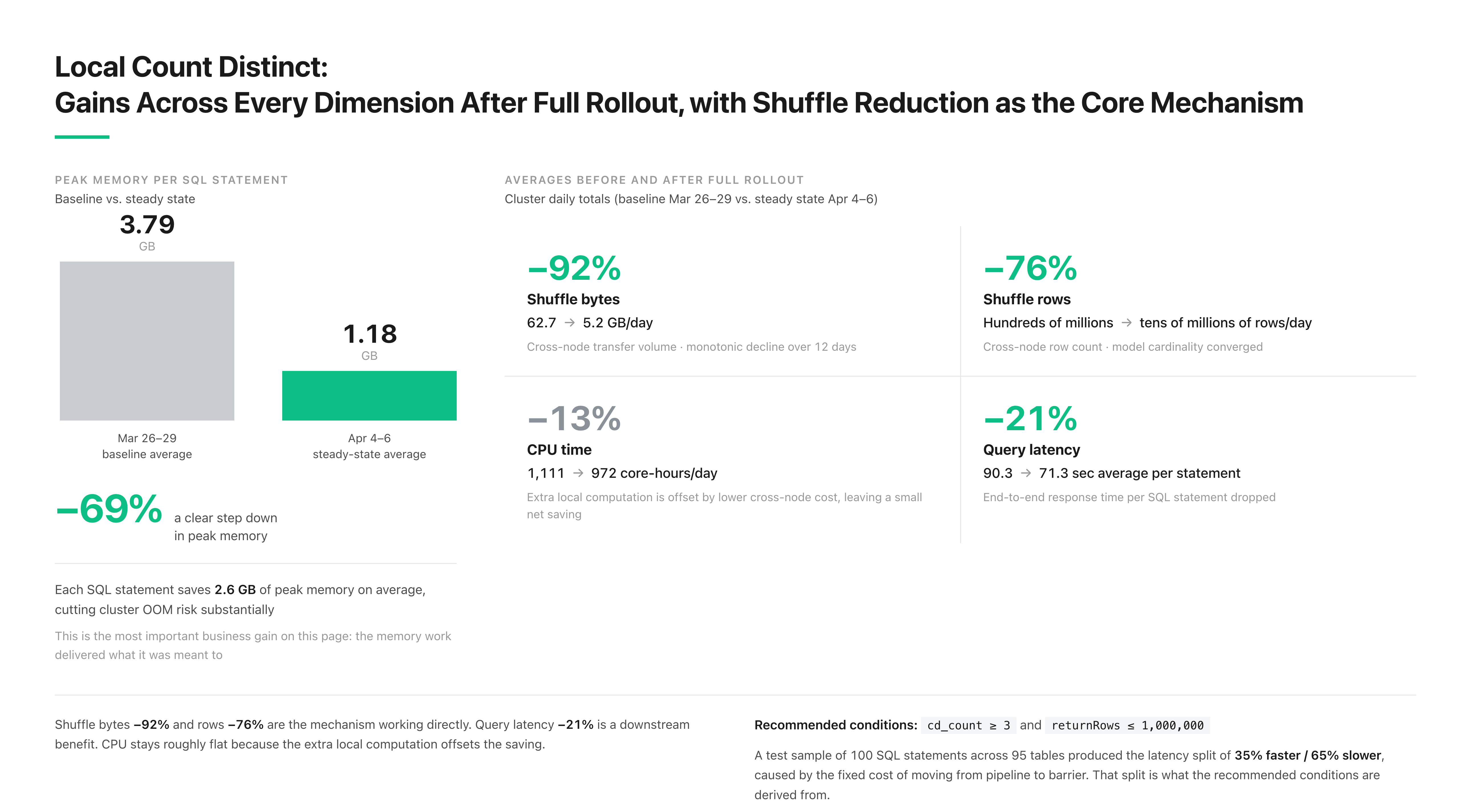
Production gains:
| Metric | Improvement |
|---|---|
| Peak memory per CU | 69% lower |
| Shuffle bytes | 92% lower |
| Shuffle rows | 76% lower |
| Query latency | 21% lower |
| CPU time | 13% lower |
One caveat: this optimization does not beat the original execution plan in every case. Native COUNT DISTINCT can compute and transmit during the shuffle, giving it some overlap between computation and network transfer. The Local rewrite has to finish local deduplication before global aggregation begins, which introduces a barrier wait of about 6 seconds.
The rewrite therefore works best where shuffle is the dominant bottleneck, such as high-cardinality Grouping Sets combined with Distinct. Whether to enable it comes down to the profile and the actual execution plan.
Compute: native C++ UDFs
Colocate Join and the Local Distinct rewrite removed most of the data movement. The next bottleneck in the profile was CPU. The assignment UDF holds the central logic of the A/B pipeline. For each user behavior log row, it determines whether that UID belongs to the experiment group, the control group, or a strategy group.
A single call costs almost nothing, in the nanosecond range. Across tens of billions of log rows, the UDF became a textbook CPU hot path.
Profile analysis showed the Java UDF taking roughly 80% of CPU, with JVM call overhead and object creation as the main bottlenecks. The team rewrote it as a C++ native UDF, eliminating Java Native Interface (JNI) call cost, then went further into the standard template library (STL) layer to optimize hot spots in memory allocation, hash access, and object construction.
The main optimizations:
-
P0, string concatenation. The original implementation created a String object per row, accounting for about 30% of CPU. The team switched to a ThreadLocal reusable fixed buffer, cutting per-row memory allocation and GC pressure.
-
P1, experiment configuration access. The original implementation looked up experiment configuration through an unordered map on every row, paying hash computation and pointer chasing. The team expanded the configuration into an array structure at initialization, giving O(1) indexed access during execution.
-
P2, user object construction. The original implementation built a smart pointer and an object instance per row, adding heap allocation and reference counting. The team switched to reading raw values directly from Block column data, avoiding the object wrapper.
Two principles ran through all three of these optimizations: remove heap allocation from the hot path wherever possible, and move repeated computation and lookups out of the loop and into initialization.
Combined, the three optimizations improved overall A/B template execution performance by about 3x.
Scheduling: holding SLAs with isolation, backpressure, and priority queues
Once Apache Doris started to carry hundreds of thousands of tasks per day, SQL-level and compute-level optimization alone was no longer enough to guarantee overall stability. The team added system-level governance at the scheduling layer.
The first layer is physical isolation. The team split the A/B cluster into 12 independent compute groups, running workloads of different priorities in different groups, each with its own resource quota. A traffic spike in a low-priority task can no longer take resources from high-priority work, which removes cross-business interference.
The second layer is in-group control, which stacks three mechanisms inside a single compute group:
-
Concurrency limits: cap the number of tasks running concurrently, queueing the rest, so a burst does not hit the cluster all at once.
-
Upstream backpressure: adjust task submission rate dynamically based on live load, keeping write and submission pace matched to what the cluster can process.
-
Priority queue scheduling: split traffic across four queues, P1 through P4, running high-priority queues first, so a backlog in a low-priority queue does not delay high-priority scheduling.
Physical isolation holds the resource boundary between groups, and in-group control keeps a single group stable. Together they keep high-priority pipelines within SLA during peak hours.
Stability: governing metadata at scale
With performance optimization done, a subtler bottleneck emerged: metadata stability.
Capacity modeling
The Apache Doris FE manages metadata, holding databases, tables, partitions, transactions, and tablet information in JVM memory. To stay recoverable after a crash, the system appends write operations to an Edit Log continuously and periodically writes a Checkpoint Image to disk, then recovers on restart by replaying the image plus a small amount of Edit Log. Running this in production exposed two risks:
-
Single-table risk. Once a single table grew past 10,000 partitions, the FE had to traverse the full partition list when generating a checkpoint. The internal structure used a Java int index, which hit its limit and caused the process to exit abnormally, disrupting the production pipeline.
-
Cluster-level risk. As table count kept growing and tablets reached tens of millions, FE metadata objects accumulated on the heap. Master FE peak memory approached the 400GB ceiling and triggered Full GC frequently.
The team moved from reactive fixes to active governance, introducing metadata capacity modeling and monitoring. On average, a single tablet occupies about 11KB in FE memory. That number gave the team a working rule. The model maps tablet growth directly onto a memory growth trend, which lets the team predict FE memory pressure in advance and keep expansion controlled.
FE optimization: smaller metadata, steadier GC, faster recovery
Beyond capacity governance, the team compressed the metadata structures themselves.
The original Table Inverted Index was designed for local storage and carried redundant fields such as local data path and local meta path. In cloud storage, those fields take no part in computation, so they become pure memory overhead.
The team introduced a Cloud Table Inverted Index, trimming fields unused in cloud deployments and replacing some collection structures with compact arrays to lower per-object cost. In a stress test at one million tablets, the optimization brought metadata memory from 4.16GB down to 1.49GB, a 64% reduction. At ten million tablets, it saves tens of GB during checkpoint peaks.
Compressing the structures shrank the footprint. How the JVM manages that footprint needed work too. FE metadata, the catalog, and Edit Log checkpoint objects are long-lived and sit mainly in the old generation. On a large heap, Mixed GC region selection, young generation ratio, and initiating heap occupancy percent (IHOP) trigger pacing all need re-tuning; otherwise the old generation keeps growing until it triggers Full GC.
The team tuned G1 GC parameters specifically for an FE running on a heap of roughly 400GB:
| Parameter | Purpose |
|---|---|
| -XX:ParallelGCThreads=48 | Match physical core count |
| -XX:ConcGCThreads=12 | ParallelGCThreads / 4 |
| -XX:G1MixedGCLiveThresholdPercent=85 | Raised from 65 to 85: accept reclaiming a region for only 15% garbage, so old-gen regions with high survival rate can still be selected by Mixed GC |
| -XX:InitiatingHeapOccupancyPercent=45 | Trigger concurrent marking at 45%, controls when it starts |
| -XX:-G1UseAdaptiveIHOP | Disable adaptive IHOP: on a large heap, long-tail traffic easily misleads it into raising the threshold |
| -XX:G1NewSizePercent=5 | Young generation floor, 5% |
| -XX:G1MaxNewSizePercent=25 | Young generation ceiling, 25% (keep it small on a large heap) |
| -XX:G1ReservePercent=20 | Reserve 20% to prevent to-space exhaustion and keep humongous allocation safe |
After tuning, 24 hours of production validation showed Master FE peak memory dropping from 370GB to 270GB, with no Full GC during the period.
Finally, the team parallelized FE startup recovery. The original flow loaded metadata serially during the loadDb phase, which took about 17 minutes at a scale of one million tables, with total startup recovery around 27 minutes. Loading table metadata in parallel cut that phase substantially and brought the overall FE recovery window down to about 10 minutes.
Canary testing results in production:
| Configuration | Total startup | Speedup | loadDb phase |
|---|---|---|---|
| Serial (before optimization) | 27.2 min | — | 17.2 min |
| 8-way parallel | 15.4 min | 1.77x | 5.8 min |
| 16-way parallel (fully rolled out) | 10.4 min | 2.61x | 4.7 min |
Taken on its own, the loadDb phase went from 17.2 to 4.7 minutes, a 3.6x gain, which cut total startup time by 62%.
As Apache Doris deployments grow, metadata governance becomes an architectural concern that belongs to system design from the start. Capacity models, lifecycle planning, and recovery capability are all part of running a large production system reliably.
Summary
Kwai's A/B metrics production reached a peak performance gain of 145x and a 72% reduction in resource consumption after upgrading from Spark to Apache Doris. Part of that came from Doris's advantage in architecture: asynchronous pipeline execution, a vectorized compute engine, and a high-performance C++ runtime.
The rest came from Kwai's own deep optimization for the A/B scenario: Colocate Join, the Local Distinct Grouping Sets rewrite, native C++ UDFs, resource isolation through physical compute groups plus logical priority queues, and metadata governance that kept the FE stable at cluster scale.
Running this at production scale confirms that Apache Doris suits the workload, and it gives the community a reference implementation for building an A/B testing platform on Doris.
Kwai also set a new record for the largest single Apache Doris cluster running in production, at 2,000 nodes and 100,000 CUs. That answers a lot of open questions about how far a single Doris cluster scales, and it leaves considerable headroom for most deployments.
For more on A/B metrics production, other use cases, and Doris deployment and optimization, join the Apache Doris community on Slack to talk with us. For a fully managed Apache Doris service, check out VeloDB.