


When designing a database schema, one of the fundamental decisions is normalization vs. denormalization.
The choice between normalized vs denormalized data directly impacts data consistency, query performance, scalability, and system architecture.
At a high level:
- Normalization reduces redundancy and improves data integrity.
- Denormalization improves read performance by reducing JOIN operations.
Understanding when to use denormalized vs normalized models depends on workload, system design, and performance goals.
| Aspect | Normalized Data | Denormalized Data |
|---|---|---|
| Goal | Reduce redundancy | Improve read performance |
| Data structure | Multiple related tables | Fewer, wider tables |
| Query pattern | JOIN-heavy | Scan-heavy |
| Storage efficiency | Higher | Lower (more duplication) |
| Best for | OLTP systems | OLAP / analytics systems |
- Choose normalization for transactional consistency.
- Choose denormalization for analytical speed.
What Is Normalization?
 Before comparing normalized vs denormalized data, it’s important to clearly understand what normalization actually means in database design.
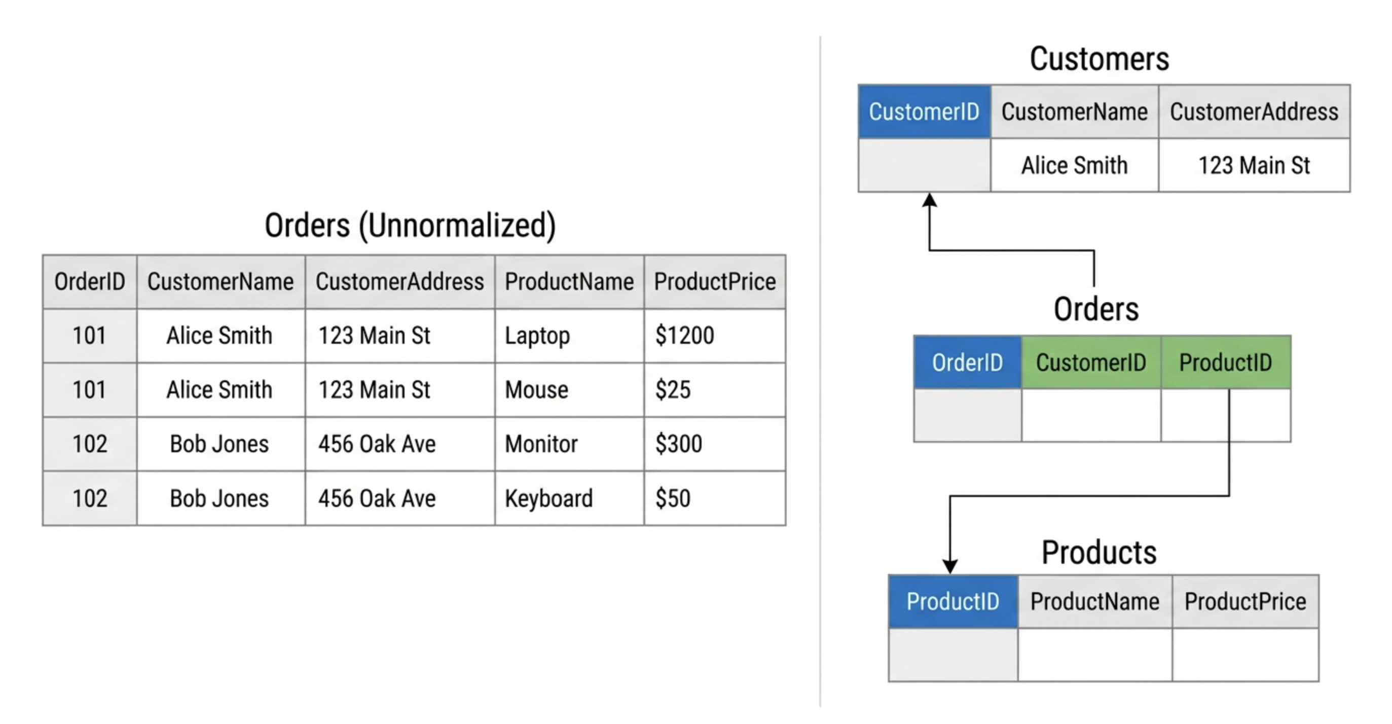
Database normalization is the process of organizing data into multiple related tables to reduce redundancy and maintain data integrity.
Instead of storing repeated information in a single large table, normalization separates entities into distinct tables and links them using primary and foreign keys. This ensures that each piece of information is stored only once, while relationships between entities are explicitly defined.
For example, instead of storing customer information repeatedly in every order record, a normalized schema would:
- Store customer data in a
Customerstable - Store order data in an
Orderstable - Link them through a customer ID
This structural separation is what makes normalized systems consistent and reliable.
Why Normalize Data?
The primary motivation behind normalization is data correctness.
When data is duplicated across multiple rows or tables, inconsistencies inevitably arise. Updating one record but forgetting another creates anomalies that are difficult to detect and fix.
Normalization helps:
- Avoid data duplication
- Maintain data integrity
- Reduce update, insert, and delete anomalies
- Improve consistency in transactional systems
There are three classic types of anomalies normalization prevents:
- Update anomaly – Changing duplicated data requires multiple updates.
- Insert anomaly – You cannot insert certain data without inserting unrelated data.
- Delete anomaly – Deleting a row accidentally removes unrelated information.
Because of these guarantees, normalization is commonly used in OLTP (Online Transaction Processing) environments such as:
- Banking systems
- CRM platforms
- ERP systems
- E-commerce checkout systems
In these systems, correctness and consistency are more important than raw query speed.
The Normal Forms Explained
Normalization is implemented through a series of design rules known as normal forms. Each normal form eliminates a specific type of redundancy or dependency problem.
Most practical database schemas aim for Third Normal Form (3NF) or Boyce-Codd Normal Form (BCNF).
1NF (First Normal Form)
A table is in 1NF if:
- It eliminates repeating groups
- Each column contains atomic (indivisible) values
- Each row is uniquely identifiable
In practice, this means no arrays or nested structures in relational columns.
2NF (Second Normal Form)
A table is in 2NF if:
- It is already in 1NF
- All non-key attributes depend on the full primary key
This removes partial dependencies, which commonly occur in composite keys.
3NF (Third Normal Form)
A table is in 3NF if:
- It is already in 2NF
- It removes transitive dependencies
In other words, non-key attributes must depend only on the primary key — not on other non-key columns.
This is the level where most transactional schemas stabilize.
BCNF (Boyce-Codd Normal Form)
BCNF is a stronger version of 3NF.
It requires that:
- Every determinant in the table must be a candidate key
BCNF addresses certain edge cases not fully covered by 3NF, particularly in complex relational structures.
In real-world engineering practice, most systems stop at 3NF or BCNF because:
- Further normalization (4NF, 5NF) increases complexity
- The marginal benefit often does not justify the additional joins
At this stage, the database is considered logically sound and protected against common redundancy issues — forming the foundation of a well-structured normalized system.
What Is Denormalization?
 If normalization focuses on reducing redundancy and enforcing data integrity, denormalization takes a different approach.
Instead of minimizing duplication, denormalization deliberately restructures data to optimize for performance — particularly read performance. To understand this shift, we first need a precise definition.
Denormalization is the process of intentionally introducing redundancy into a database by merging tables or duplicating data to improve read performance.
Rather than storing each entity in separate normalized tables, denormalization combines related data into fewer, wider tables. This reduces the need for expensive JOIN operations during query execution.
In other words:
- Normalization optimizes for data correctness and storage efficiency.
- Denormalization optimizes for query speed and analytical simplicity.
Instead of reducing redundancy, denormalization trades storage efficiency for faster reads and simpler query execution.
Why Denormalize Data?
While normalization protects consistency, it can introduce performance costs — especially in large-scale or distributed systems.
In normalized schemas, answering a single query may require multiple JOIN operations. In distributed databases, these JOINs often trigger:
- Data shuffling across nodes
- Network transfer overhead
- Large intermediate result sets
- Increased query latency
Denormalization is often used to:
- Reduce JOIN cost
- Improve read-heavy query performance
- Support analytical workloads
- Simplify query logic
- Minimize cross-node data movement
This is especially common in OLAP (Online Analytical Processing) systems, where:
- Queries scan large datasets
- Aggregations are frequent
- Writes are less frequent than reads
In analytics environments, eliminating JOINs can significantly improve performance — particularly for dashboards, reporting, and customer-facing analytics.
Common Denormalization Techniques
Denormalization is not random duplication. It is typically applied using specific design strategies.
Common techniques include:
- Table merging – Combining related tables into a single wide table
- Pre-aggregated tables – Storing computed metrics in advance
- Materialized views – Persisting query results for reuse
- Star schema (fact + dimension tables) – Flattening dimension data for analytical efficiency
- Wide tables for analytics – Creating read-optimized structures for serving queries
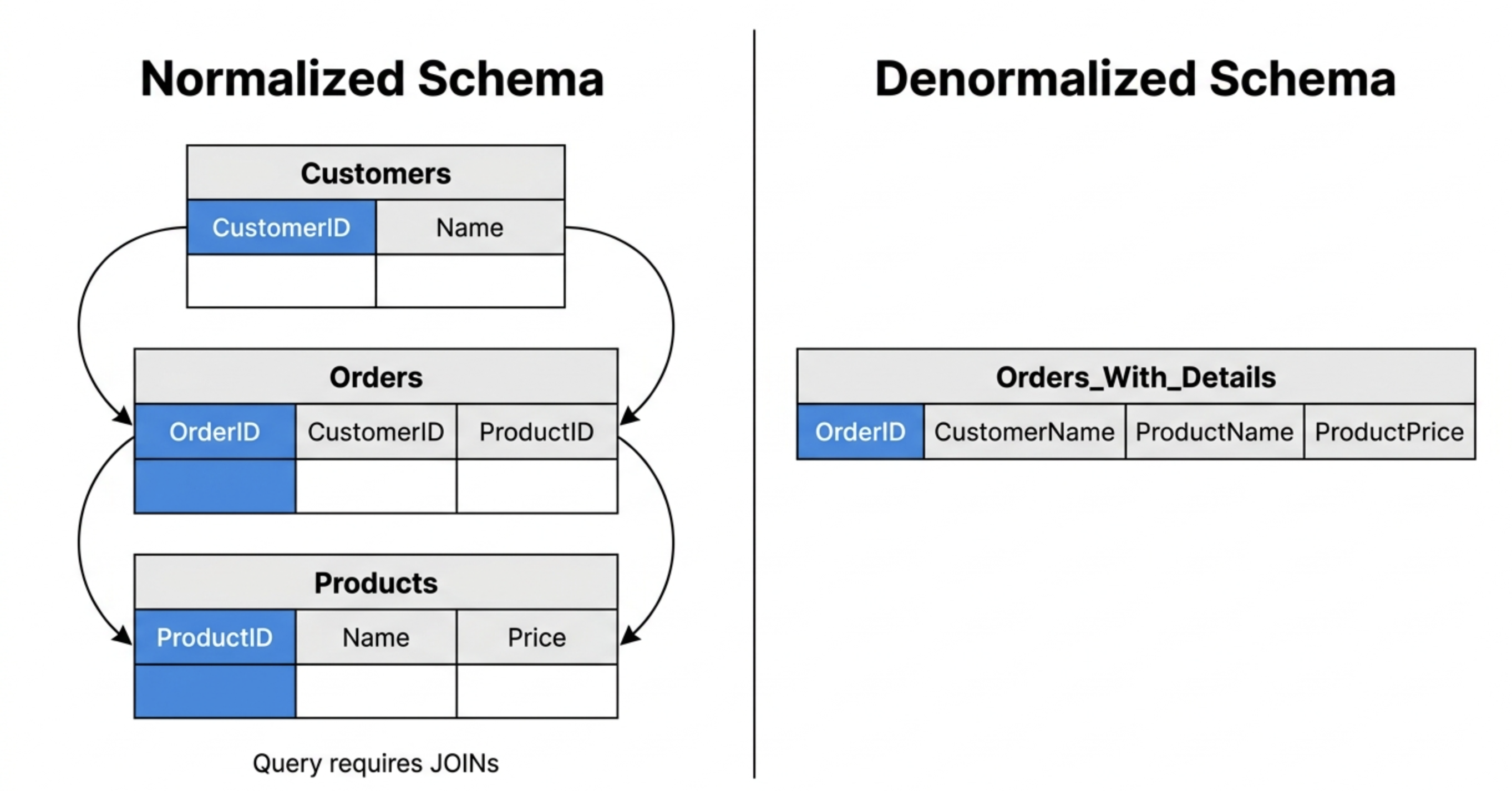
For example, instead of joining Orders, Customers, and Products at query time, a denormalized schema may pre-join these into a single analytics table.
This shifts complexity from query time to data modeling time.
Importantly, denormalization is often a deliberate optimization step, not a default design choice. Many systems begin with a normalized schema and selectively denormalize performance-critical workloads.
In modern analytical engines — especially distributed, columnar systems — the decision between normalized vs denormalized data becomes less absolute. Some engines can efficiently execute distributed JOINs, reducing the need for aggressive denormalization.
That’s why the real question is not simply denormalized vs normalized, but rather:
What workload are you optimizing for?
Normalized vs. Denormalized Data
After understanding what normalization and denormalization mean individually, the next step is to compare them directly.
A side-by-side view makes it easier to see how normalization vs denormalization differs across storage design, performance characteristics, and workload patterns.
Here is a more engineering-focused comparison of normalized vs denormalized data:
| Dimension | Normalization | Denormalization |
|---|---|---|
| Data redundancy | Minimal — data stored once | Increased — data intentionally duplicated |
| Write consistency | Strong — fewer anomalies | More complex — duplication must be synchronized |
| Read performance | Slower (JOIN-heavy queries) | Faster (scan-heavy queries) |
| Query complexity | Higher — requires JOIN logic | Lower — simplified query patterns |
| Storage usage | Efficient | Higher due to redundancy |
| Scaling pattern | Optimized for transactional integrity | Optimized for read scalability |
| Typical system | OLTP systems | Data warehouses / analytics platforms |
What This Comparison Really Means
This table highlights an important point:
The debate around normalized vs denormalized is fundamentally a tradeoff between:
- Consistency and storage efficiency vs. Query performance and simplicity
In normalized schemas:
- Data integrity is prioritized.
- Writes are safer and easier to maintain.
- Reads may require multiple JOIN operations.
In denormalized schemas:
- Reads are simplified.
- Aggregations are faster.
- Storage and update complexity increase.
This is why the decision between normalization vs denormalization depends heavily on workload type:
- Transaction-heavy systems favor normalization.
- Read-heavy analytical systems often favor denormalization.
However, modern distributed, columnar engines are narrowing this gap. With improved JOIN execution, vectorized processing, and cost-based optimization, some platforms can efficiently support both denormalized vs normalized models within the same architecture.
In practice, the question is no longer:
Which one is correct?
But rather:
Which one better aligns with your workload characteristics and performance goals?
When to Use Normalization vs. Denormalization
Understanding the theoretical difference between normalization vs denormalization is useful — but architectural decisions are made based on workload.
The real question engineers ask is:
Given my system constraints, which model better fits my performance and consistency requirements?
Let’s break it down.
Use Normalization When…
Normalization is the right choice when data correctness and transactional integrity are your top priorities.
You should favor normalized schemas when:
- Building transactional systems (OLTP)
- High write consistency is critical
- Financial or compliance-heavy applications
- Frequent updates to individual records
- Multiple concurrent write operations occur
- Data integrity violations would be costly
Examples include:
- Payment processing systems
- Banking ledgers
- Order management platforms
- Inventory systems
In these systems:
- Writes happen frequently.
- Individual records are updated often.
- Preventing anomalies is more important than minimizing JOINs.
Normalization prevents update, insert, and delete anomalies and ensures that data remains consistent even under heavy write concurrency.
Use Denormalization When…
Denormalization is appropriate when read performance and query simplicity matter more than strict storage efficiency.
You should consider denormalized schemas when:
- Building dashboards or reporting systems
- Powering real-time analytics
- Running aggregation-heavy queries
- Designing data warehouses
- Serving customer-facing analytics
- Supporting read-heavy workloads with fewer updates
Examples include:
- Business intelligence dashboards
- Observability platforms
- IoT analytics systems
- Recommendation systems
- Customer-facing metrics APIs
In these environments:
- Reads significantly outnumber writes.
- Queries scan large datasets.
- Aggregations and filtering dominate workload patterns.
Denormalized schemas reduce expensive JOIN operations and simplify query logic, often resulting in lower latency for analytical queries.
Normalization vs. Denormalization in Modern Analytics Systems
Historically, OLAP systems strongly favored denormalization — and for good reason.
In early distributed database architectures, JOIN operations were expensive.
Why?
- Distributed JOINs required data shuffling across nodes
- Network transfer became a bottleneck
- Large intermediate result sets increased memory pressure
- Query latency scaled poorly with table relationships
To avoid these costs, teams flattened schemas into:
- Star schemas
- Snowflake schemas
- Wide denormalized tables
Denormalization became a performance necessity rather than a modeling preference.
What Has Changed?
Modern analytical engines have significantly altered this tradeoff.
Several architectural improvements have reduced the penalty of JOIN operations:
- Columnar storage reduces scan cost by reading only required columns
- Vectorized execution processes batches efficiently, improving JOIN throughput
- Cost-based optimizers minimize unnecessary data movement
- Distributed execution planning improves data locality
- Materialized views precompute expensive joins and aggregations
As a result, the binary thinking of normalized vs denormalized is becoming less rigid.
The Serving-Layer Perspective
In modern real-time analytics systems, especially those serving customer-facing applications, the requirements are more complex:
- High concurrency
- Real-time ingestion
- Mutable data (updates, not just append-only)
- Hybrid workloads (structured + full-text + vector queries)
Advanced real-time analytics platforms like VeloDB, built on Apache Doris, are designed to handle both normalized and denormalized workloads efficiently.
Because VeloDB supports:
- High-performance distributed JOINs
- Real-time upserts (mutable analytics)
- Columnar storage with vectorized execution
- Native inverted indexes
- Native vector indexes
- Hybrid search + analytics
Teams no longer have to fully commit to denormalized-only schemas for performance.
Instead of restructuring schemas purely to avoid JOIN cost, engineers can:
- Start with logically clean models
- Benchmark real workloads
- Apply selective denormalization only where necessary
- Use materialized views or indexing strategies strategically
This significantly reduces the traditional tension between normalization vs denormalization in modern serving-layer architectures.
The New Reality
The debate is shifting from:
“Which model is faster?”
to:
“Which model aligns with my workload characteristics and engine capabilities?”
In modern distributed, columnar, real-time systems, the choice between denormalized vs normalized is increasingly contextual — not absolute.
And that shift is one of the most important evolutions in database design over the last decade.
Can You Use Both? (Hybrid Modeling Strategy)
After comparing normalization vs denormalization, it may seem like you must choose one approach.
In reality, most modern systems use both.
Very few production architectures are purely normalized or purely denormalized. Instead, they apply each strategy where it makes the most sense.
Why Hybrid Modeling Is the Norm
Different layers of a data stack have different priorities:
- Transactional layers prioritize consistency.
- Analytical layers prioritize query performance.
- Serving layers prioritize latency and concurrency.
As a result, real-world architectures often look like this:
- Operational databases remain normalized (often 3NF or BCNF).
- Analytics layers introduce selective denormalization (fact tables, aggregates).
- Serving layers support mixed workloads, depending on query patterns.
For example:
- An OLTP database stores orders, customers, and products in 3NF.
- A reporting system maintains aggregated fact tables.
- A real-time serving layer powers dashboards or customer-facing analytics with optimized views.
This hybrid strategy allows teams to:
- Preserve data integrity in core systems.
- Optimize read-heavy queries where needed.
- Avoid unnecessary redundancy in transactional layers.
Selective Denormalization vs. Over-Denormalization
A common mistake is to over-denormalize too early.
Aggressive denormalization can:
- Increase storage costs
- Complicate update logic
- Create synchronization challenges
- Introduce data drift between duplicated fields
Modern best practice is often:
Start normalized, then denormalize selectively based on measured bottlenecks.
In distributed analytical engines, especially those with efficient JOIN execution, you may not need to flatten everything upfront.
Modern systems increasingly blur the boundary between denormalized vs normalized strategies — allowing schema clarity and performance optimization to coexist.
FAQ — Normalization vs. Denormalization
Below are common questions engineers ask when evaluating normalized vs denormalized data.
What is the difference between normalized vs denormalized data?
- Normalized data minimizes redundancy by splitting data into multiple related tables connected through keys.
- Denormalized data combines related data into fewer tables to reduce JOIN operations and improve read performance.
The core difference in normalization vs denormalization lies in whether you optimize for integrity or query speed.
Is denormalized vs normalized better for analytics?
Traditionally, denormalized schemas perform better for analytics because they reduce JOIN cost.
However, modern columnar and distributed engines can efficiently execute JOINs. In these systems, normalized models may still perform well, especially with proper indexing and query optimization.
The better approach depends on workload size, concurrency, and engine capabilities.
Does denormalization always improve performance?
Not always.
Denormalization typically improves read-heavy, aggregation-focused workloads. But it can:
- Increase storage usage
- Complicate updates
- Introduce consistency challenges
- Slow down write-heavy systems
Performance gains depend on query patterns and system architecture.
Can normalization hurt performance?
Yes — in certain contexts.
In distributed systems, excessive normalization can:
- Increase JOIN operations
- Trigger cross-node data shuffling
- Create large intermediate datasets
If JOIN execution is inefficient, normalized schemas may increase latency.
Why is normalization important in OLTP systems?
Normalization ensures:
- Strong data consistency
- Reduced redundancy
- Protection against update, insert, and delete anomalies
- Easier transactional control
For systems where correctness is critical (e.g., financial records), normalization is essential.
Why is denormalization common in data warehouses?
Data warehouses are read-heavy and aggregation-driven.
Historically, distributed JOINs were expensive, so flattening schemas improved query speed. Star schemas and wide tables reduced runtime JOIN cost and simplified BI queries.
That’s why denormalization became common in analytical environments.
Can normalization and denormalization coexist in the same system?
Yes — and they often do.
Many modern architectures:
- Store operational data in normalized form
- Build denormalized views for analytics
- Use materialized views for performance-critical queries
This layered strategy balances integrity and performance.
How do modern analytics engines change the decision?
Modern distributed engines with:
- Columnar storage
- Vectorized execution
- Cost-based optimization
- Efficient distributed JOIN algorithms
Reduce the performance penalty of normalized schemas.
As a result, the strict divide between normalized vs denormalized is becoming less rigid.
The better question today is:
What modeling strategy best aligns with your workload and system capabilities?
Conclusion
The debate around normalization vs denormalization is not about right or wrong.
It’s about workload.
- Transactional systems prioritize integrity → normalization
- Analytical systems prioritize performance → denormalization
But modern distributed, columnar, real-time engines are reducing the historical tradeoffs.
Instead of choosing strictly between normalized vs denormalized data, modern architectures increasingly support both — allowing engineers to design schemas around clarity and workload patterns rather than rigid constraints.
Understanding this balance is key to building scalable data systems.