


The database landscape has cycled through several waves of specialization and consolidation. New needs spur innovation, creating specialized databases that then evolve to address broader operational burdens. VeloDB and Apache Doris have followed this exact trajectory: born as a specialized database for real-time analytics, they have evolved to support full-text search, data warehousing at scale, and now serve as a knowledge store for Generative AI.
At the heart of every database evaluation is performance. However, different use cases demand different performance profiles, and the devil is always in the details. This blog series provides relevant performance data for the typical use-case patterns supported by VeloDB.
In this first installment of the VeloDB Performance Benchmark Series, we will dive into the use case that started it all: Real-Time Online Analytics Processing. We will define the scope of "real-time", identify the critical SLAs for real-time analytics, and explore the technical architecture of VeloDB that supports those critical SLAs.
What is Real-Time Analytics?
"Real-time" is often an ambiguous term. For the scope of this benchmark, we define real-time analytics as querying data within a 1–5 second window of its generation. A use case that performs real-time analytics can be a live dashboard monitoring stock trades or user activity. In these scenarios, the system must ingest massive data streams while simultaneously serving thousands of concurrent users with sub-second response times.
The 3 SLAs that matter for real-time analytics
To truly evaluate a real-time system, we must look beyond just query latency, data freshness, query concurrency, and join performance are also important for real-world situations
1. Data Freshness
This is the holy grail of real-time analytics. It measures the time elapsed from the moment an event occurred to the time that data is made available in a query. Typically, this is evaluated by looking at query latency under heavy database updates.
2. Query Concurrency
Concurrency measures how many simultaneous users a system can handle without degradation. In customer-facing apps, user counts can spike into thousands. The system must remain performant under high load to maintain strict real-time SLAs. This is evaluated by examining queries per second under different parallelization scenarios.
3. Join Performance
Real-world data is rarely a single flat table. It usually exists in structured relational tables like a Star Schema. When data is frequently updated across multiple tables, the database must perform complex joins on the fly without sacrificing freshness.
Benchmarks
The benchmarks that will be used to evaluate the three SLAs above will be Star Schema Bench and ClickBench. For each test, there will be specific hardware set ups that are normalized between the comparisons.
Data Freshness Benchmark
For data freshness, the Star Schema Bench SF-100 is used. The data volume is around 100GB. For the hardware setup, a 16 Core 128GB compute node was used for the VeloDB deployment, and a 32-core 128GB ClickHouse deployment (2 replicas, each replica has 16core CPU and 64GB of Memory) is used. For ClickHouse, the ReplacingMergeTree configuration is used to achieve "real-time updates". Additionally, two update scenarios were tested, one with 25% of the data being updated and the other 100% of the data being updated.
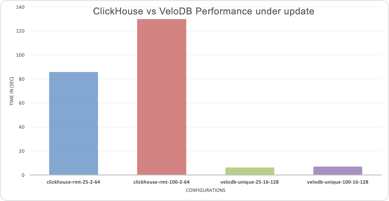
VeloDB (16c 128GB) vs. ClickHouse 32c 128GB (2 replicas, each replica 16c 64GB):
-
At 25% update ratio, VeloDB's query response time is 14X faster than ClickHouse.
-
At 100% update ratio, VeloDB's query response is 18x faster than ClickHouse.
Further details with this benchmark can be found here: Apache Doris Up to 34x Faster Than ClickHouse in Real-Time Updates
Concurrency Benchmark
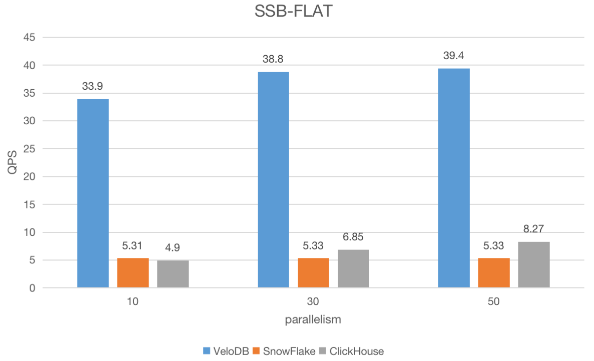
In this evaluation, we selected a 128-core hardware configuration for both VeloDB and ClickHouse Cloud. A Snowflake XL (X-Large) cluster, which is approximately equivalent to a 128-core cluster on the other 2 systems, was chosen for the benchmark.
Apache JMeter, an open-source load testing tool, was used to start 10, 30, and 50 threads and submit queries in sequence, running each query for 3 minutes, then calculating QPS for each query.
In the first concurrency test, we will query a single large table, typical of a BI setup with a high number of analysts querying denormalized data.
For this test, we used SSB-FLAT with a 100GB data volume, designed to measure a system's capacity to query a single wide table. Tables in SSB are converted into a single denormalized flat table. In this benchmark, no join operations are used.
Concurrency with Joins Benchmark
The same hardware setup for SSB-flat is used for SSB
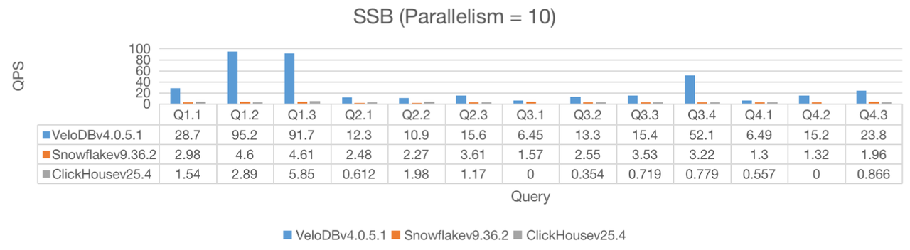
We use the Star Schema Bench (SSB) for this benchmark with 100Gig data volume. SSB was designed to test star schema optimization, and it is a simple benchmark that consists of four query flights, four dimensions, and a simple roll-up hierarchy.
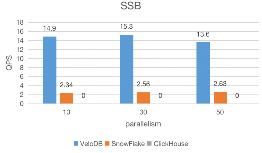
In this benchmark, VeloDB completed all 13 queries and had significantly higher QPS under all three parallelization scenarios, while Clickhouse was unable to complete all the queries.
Note: 0 value below means incomplete queries
How VeloDB Delivers Real-Time Performance
How does VeloDB achieve high freshness and low latency? It comes down to a combination of smart storage models, aggressive pruning, and a modern execution engine.
1. High Data Freshness: The Unique Key Model /Delete BitMap
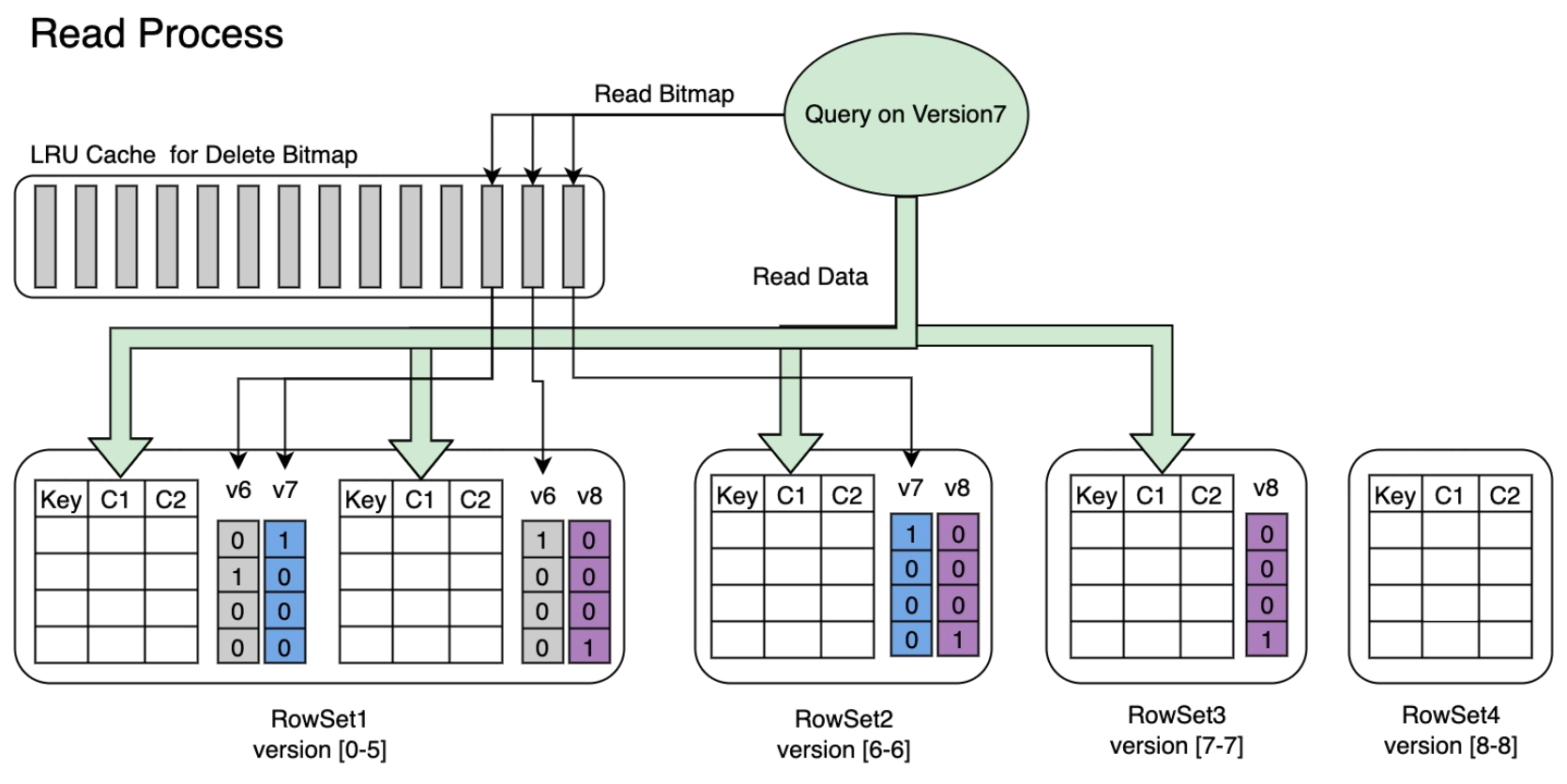
VeloDB is built with the Unique Key model, which allows tables to efficiently overwrite existing records with the same primary key. VeloDB employs a mechanism called Delete Bitmap to optimize query performance.
VeloDB's Delete Bitmap mechanism doesn't require calculating deletion logic during queries. This significantly reduces query latency, keeping response times consistently within hundreds of milliseconds, even under high concurrency.
How updates are handled?
1. Write Stage
When creating a table with the Unique Key model, you typically define a unique identifier (e.g., primary key ID) and a version column (e.g.,update_time). Whenever new data is written, if the primary key matches and the version is newer, VeloDB automatically marks the old data with a "delete mark." This information is written to the underlying storage along with the data.
2. Query Stage
During query execution, VeloDB automatically identifies and skips data rows marked for deletion, eliminating the need to compare or scan multiple versions of data. This enables low-latency, high-efficiency data reads.
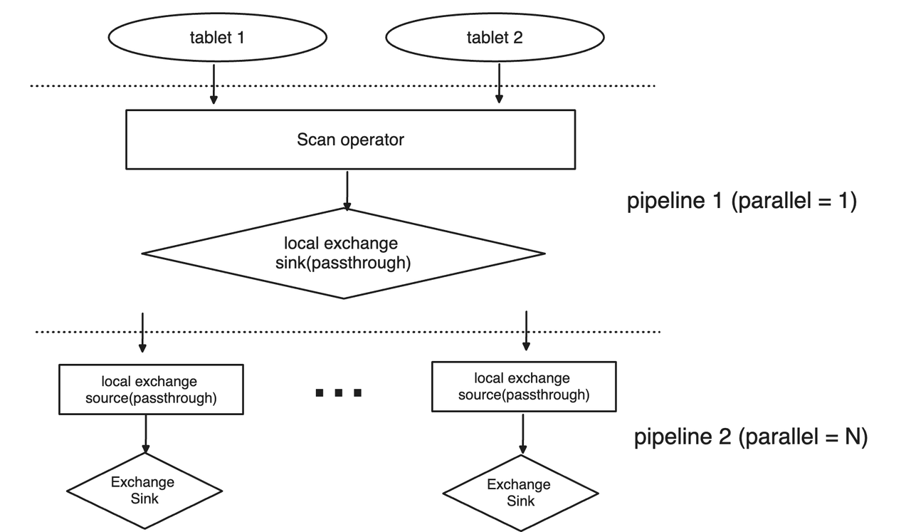
2. High Concurrency: The Pipeline Execution Engine
To handle thousands of concurrent users, VeloDB uses a Pipeline Execution Engine.
-
Non-Blocking Execution: The engine yields the CPU whenever a blocking operator is met (e.g., Disk I/O or Network I/O). This allows threads to switch to compute-intensive tasks immediately, maximizing CPU utilization.
-
Parallelism: Data is evenly redistributed across tasks to prevent skew, and parallelism is determined independently for each pipeline, ensuring that no single slow node bottlenecks the entire query.
3. Intelligent Data Pruning: Optimizing joins and analytics
The fastest way to process data is to not process it at all. VeloDB minimizes I/O by filtering out unnecessary data before it ever hits the compute layer.
-
Predicate Filtering (Static):
-
Partition Pruning: The frontend determines which partitions are required based on metadata, skipping entire blocks of data.
-
Key Column Pruning: Using the sorted order of key columns, the engine uses binary search to locate the specific range of rows needed.
-
Zone Maps: Each data file maintains max/min value metadata. If a query's predicate falls outside a file's range, the entire file is skipped.
-
-
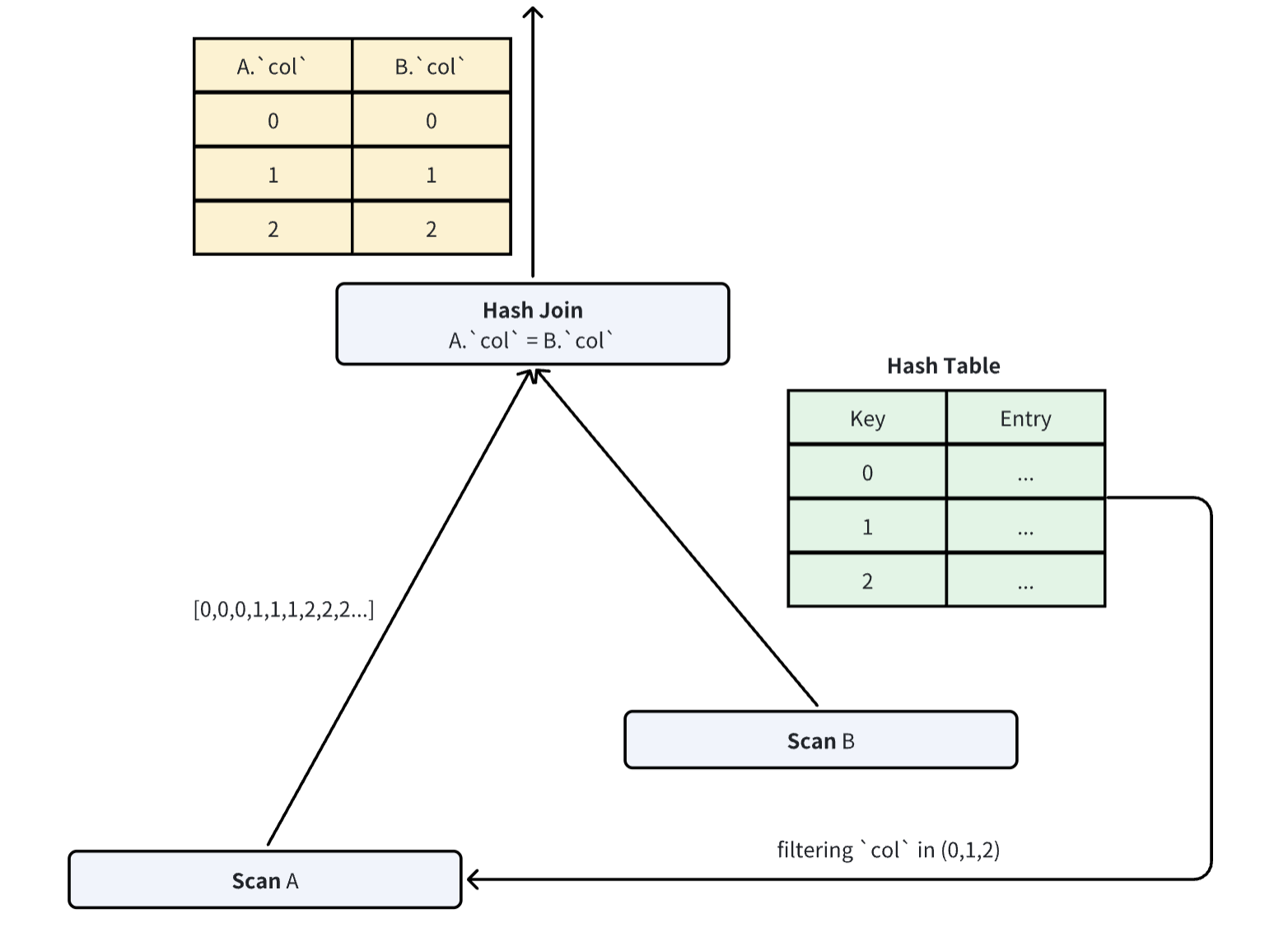
Dynamic Join Pruning (Runtime Filters): For joins, the optimizer builds a Hash Table on the smaller "Build" table first. It then generates filters dynamically to prune the larger "Probe" table. This reduces join complexity from O(M×N) to roughly O(M+N).
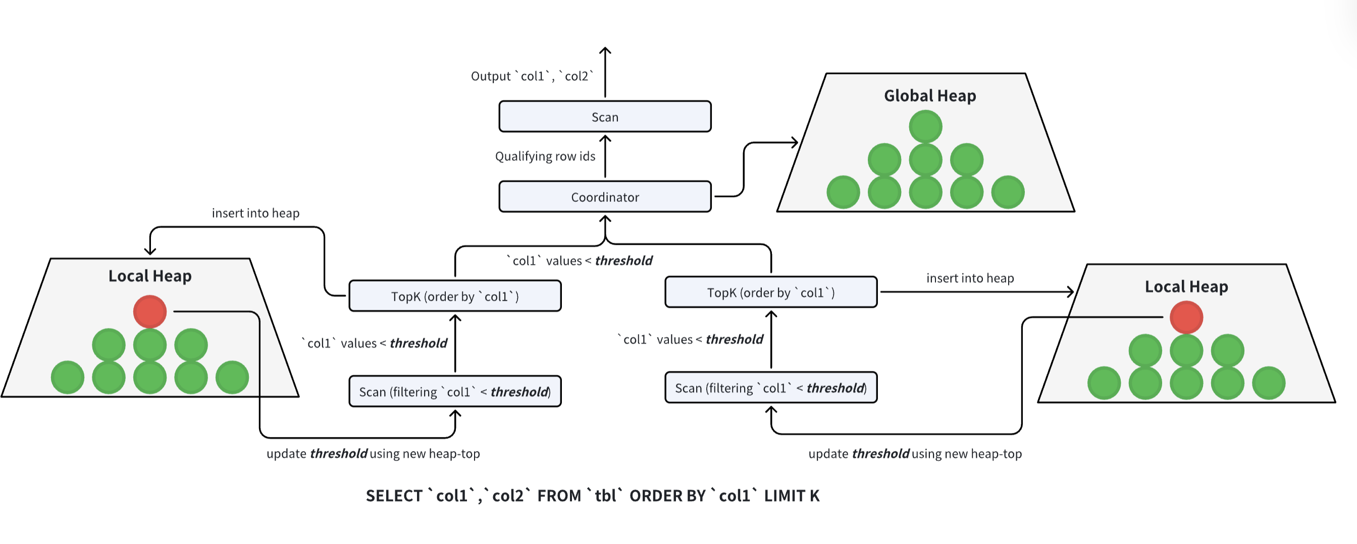
- TopK Pruning: For queries asking for the "Top 10" or "Top 100" results, VeloDB optimizes the sort phase. Instead of fully sorting all data (which is expensive), it uses a heap sort method that aggressively discards data that cannot possibly make it into the top K results during the scan phase.
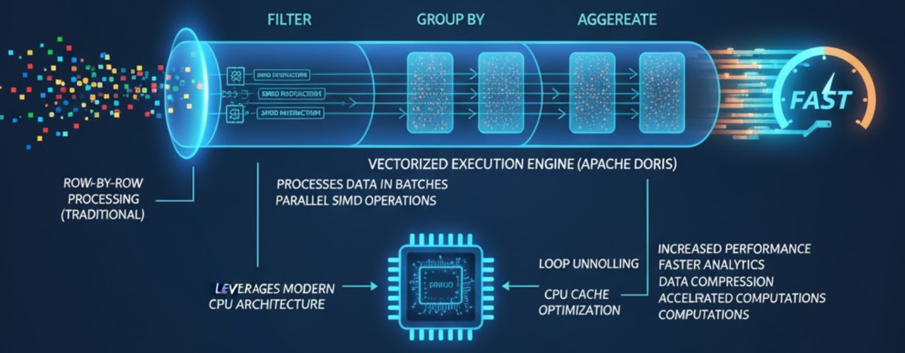
4. Vectorized Query Execution: Effective Use of Computing
VeloDB processes data in batches (vectors) rather than row-by-row. This leverages modern CPU architectures (SIMD instructions) and cache locality, significantly accelerating operations like data compression and loop computations.
Replicate the Results
Transparency is key to benchmarking. If you want to verify these results or test VeloDB against your own workloads:
-
Get the Environment: If you don't have an instance yet, try VeloDB for free today.
-
Run the Benchmarks:
In the next post of this series, we will explore Lakehouse query performance over open table formats. Stay tuned!