How to Build a Real-Time Web3 Analysis Infrastructure with Apache Doris and Flink

Web3 analytics is a race against time. When a whale wallet moves, when a rug pull begins, when market manipulation unfolds, users need to see it in milliseconds, not minutes.

But traditional data architectures can't keep up with the real-time, large-scale, relentless demands of blockchain data: popular chains like Solana and BSC are designed to handle thousands of transactions per second, and analytics dashboards must serve thousands of concurrent users querying billions of historical records.

This article walks through how to build a real-time Web3 analytics platform using Apache Doris and Apache Flink. This is a combination that delivers:

Sub-second queries on billions of transaction records (500ms–1s)
200ms latency for real-time metrics like trading volume, price, and holder stats
5,000+ QPS for high-concurrency storage and query workloads

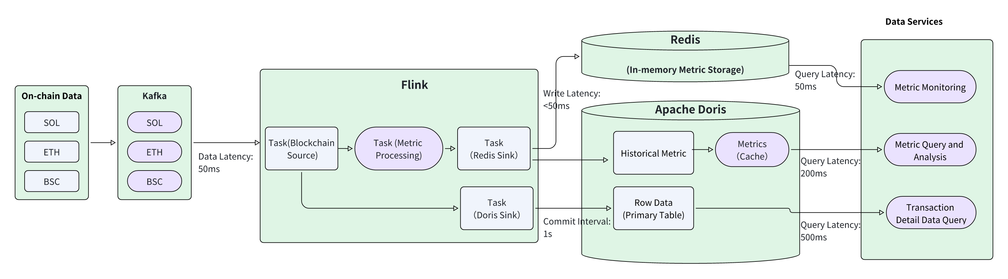
We'll cover the full architecture: Flink for real-time metric computation and Redis writes, Apache Doris for high-concurrency storage and queries, plus schema design, partitioning strategies, and materialized views for analytics.

Why Web3 Data Needs A New Architecture

Popular Blockchains and Their Characteristics

Public Blockchain	Key Features	Architectural Advantages	Ecosystem Status	Main Challenges
Ethereum	Rich smart contracts, DeFi, NFT ecosystem	Decentralized, highly compatible	Largest ecosystem, but limited scalability	High gas fees, limited TPS, network congestion
Binance Smart Chain	High speed, low cost	Compatible with Ethereum ecosystem	Rapidly growing but less decentralized	Security concerns
Solana	Ultra-high TPS, low latency	High performance, low cost	Ecosystem gradually expanding	Network stability and security challenges
GMGN	High performance, low latency, smart contract support	Designed for large-scale analytics and scenario adaptation	Emerging ecosystem, analytics-focused	Ecosystem maturity and user base need improvement

Main Use Cases

On-chain Behavior Monitoring: Real-time detection of extreme transactions and manipulative behaviors (e.g., flash crashes, money laundering).
DeFi Risk Control: Monitoring liquidity changes, lending metrics, and setting risk threshold alerts for liquidity pools.
Fund Flow Tracking: Identifying whales and tracing capital migration paths.
Social Metric Analysis: Tracking KOL wallets and community activity levels.
Market Manipulation and Bot Detection: Analyzing bundled transactions, sniper trades, and wash trading.
Ecosystem Governance and Decision-making: On-chain voting and community behavior analysis.

Industry Pain Points

Real-time Data: On-chain transactions and state changes occur rapidly and require second-level responsiveness.
Complex Algorithms and Diverse Metrics: Supporting multi-dimensional, multi-metric, and cross-analysis scenarios.
Massive Data Storage and Retrieval: Storing full-chain data while supporting high-concurrency queries.
High Flexibility: Supporting dynamic metric definitions and various analytical scripts.
Security, Privacy, and Compliance: Data access control and privacy protection solutions.

What makes Web3 data different

Extreme real-time requirements: In Web3, on-chain data moves fast. Transactions and state changes happen in an instant, and analytics platforms need to update data and compute metrics within 200ms to 1 second. This real-time capability underpins critical use cases: anti-money laundering surveillance, anomaly detection, and market manipulation alerts all depend on catching changes the moment they happen.
High concurrency at scale: Web3 applications serve thousands of users querying token prices, wallet balances, holder rankings, and transaction histories simultaneously. Data systems need to support 5,000+ QPS while keeping query latency under 200ms for responsive front-end experiences: real-time candlestick charts, live transaction feeds, instant wallet lookups. This puts serious pressure on both the storage layer's horizontal scalability and the query engine's optimization.
Complex Computation: On-chain data is inherently complex. A single transaction can involve multiple inputs and outputs, nested smart contract calls, and cross-protocol interactions. Computing meaningful metrics requires multi-dimensional analysis: tracing transaction paths, mapping fund flows, tracking position changes, and decoding contract interactions. This isn't simple aggregation—it's a multi-stage computation that demands serious processing power.
Dynamic and evolving metrics. Web3 analytics goes far beyond basic transaction counts. The real value lies in advanced indicators: net buy/sell within trading windows, top-N holder concentration, smart money tracking, whale movement detection, and manipulation pattern recognition (bundled trades, front-running, sniper attacks). These use cases evolve constantly: new tokens, new attack vectors, new signals worth tracking. Platforms can't hardcode every metric; they need flexibility to define new indicators and adjust logic without re-engineering the pipeline.

Solution: Real-time architecture based on Flink + Apache Doris

Apache Doris and Flink Solution Summary

Flink, Real-Time Metrics Engine: Flink handles real-time computation. It subscribes to blockchain data from Kafka with low latency, parses the raw data, and computes metrics on the fly. Hot metrics are written to Redis in real-time, enabling high-concurrency lookups for live dashboards. Meanwhile, Flink sends both computed metrics and transaction details to Apache Doris via Stream Load, building up the historical data layer for deeper analysis.
Apache Doris, High-Concurrency Query and Analytics: Apache serves as the storage and query backbone. Data is organized using time-based partitioning and token address bucketing for optimized storage and retrieval. With partitioning, bucketing, and inverted indexes working together, Apache Doris delivers detailed transaction queries across tens of billions of rows in 500ms to 1 second, and aggregated metrics queries at around 200ms, even under high concurrency. The primary key model ensures global deduplication, preventing duplicate records from polluting your dataset.
Metric Processing: For aggregated statistics, Apache Doris's built-in materialized views handle the heavy lifting. This keeps metrics computation inside the database, eliminating the need for external ETL jobs. The result: a unified platform where both real-time metrics and detailed transaction queries live in one place.

1. Apache Doris and Flink

A. Flink for Real-time Metrics Calculation

Leveraging Flink's high-performance real-time computing capabilities, continuous transaction data on public blockchains is processed to generate real-time metrics within milliseconds to seconds. The specific computation process is as follows:

Data Collection: Consume public blockchain data in real time from Kafka, with typical latency around 50ms.
Data Parsing and Metric Processing: Parse on-chain data and process real-time metrics. Common metrics include real-time transaction volume, open price, close price, high price, low price, etc. Metrics are calculated once per second and written into Redis.
Real-time Metrics Service: Redis Sink writes real-time metrics into Redis. Real-time monitoring services query Redis to obtain the latest metrics for each token, providing up-to-date monitoring indicators. Using Redis's high-concurrency capabilities, high-concurrency, low-latency metric queries are achievable.
Transaction Detail Storage: Doris Sink ingests transaction details into Doris for detailed transaction and statistical data analysis.

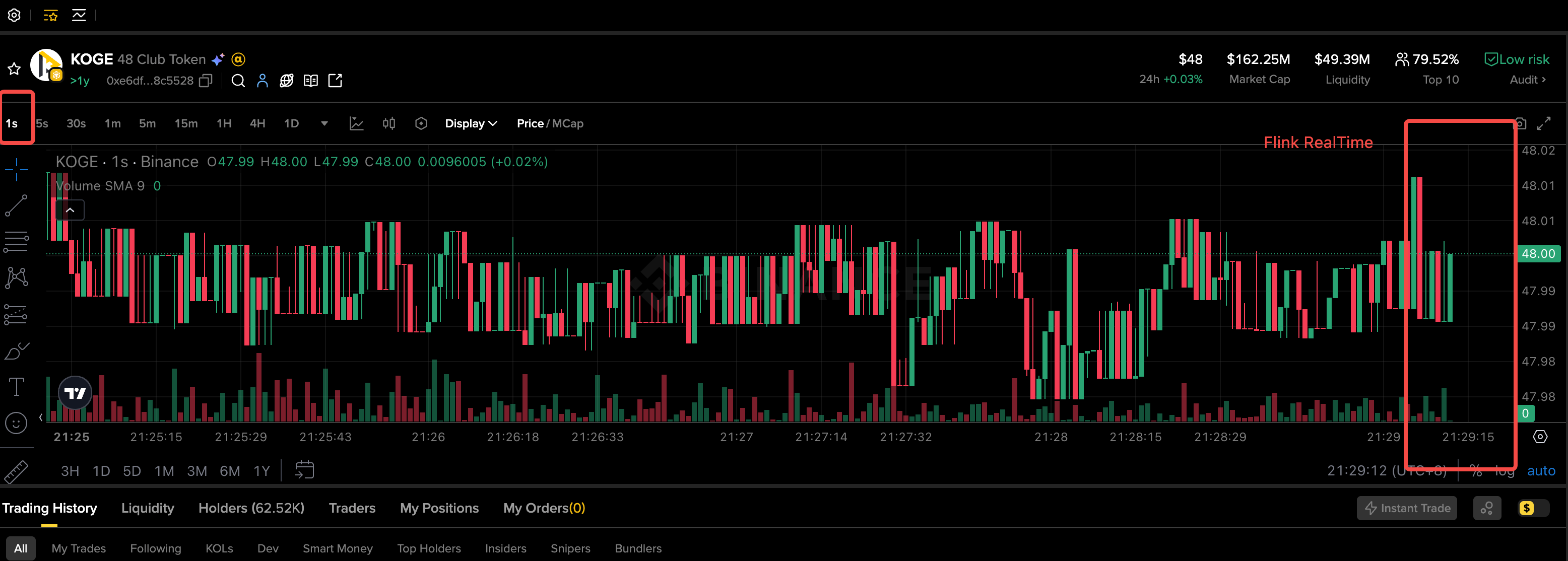
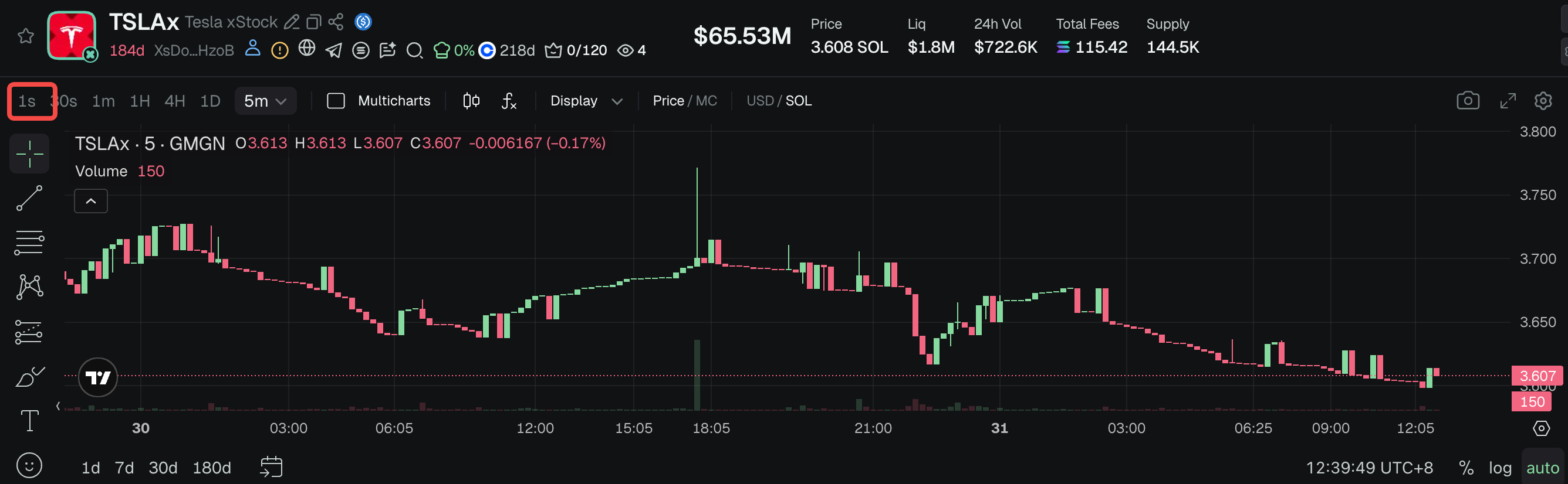
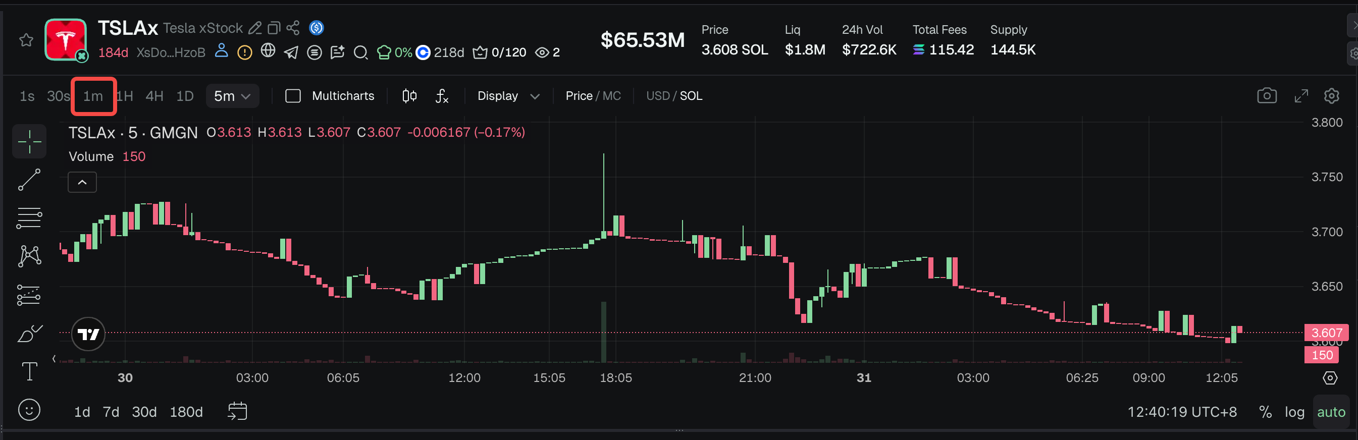
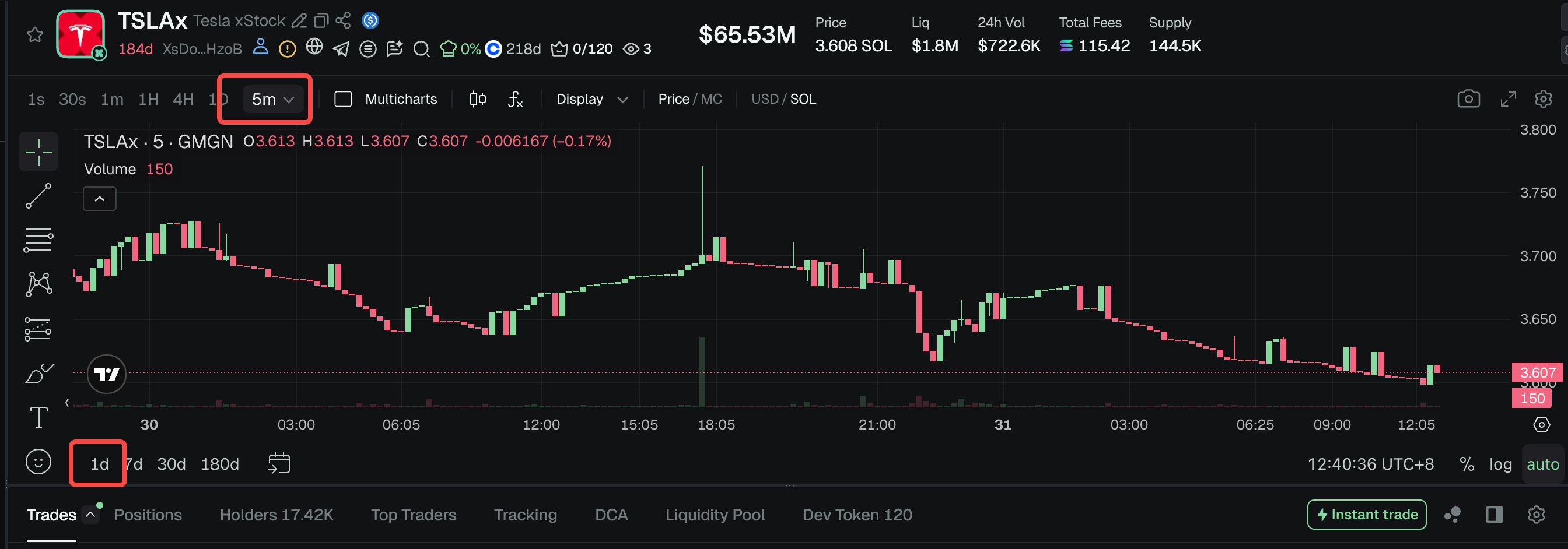
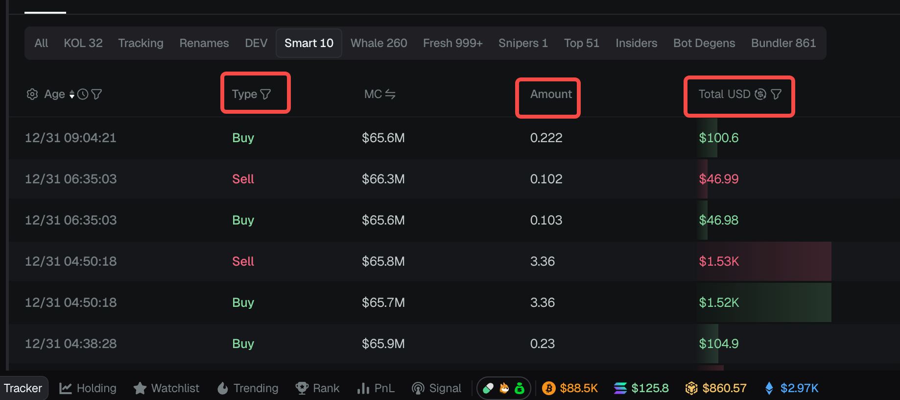
By leveraging the Flink real-time computing engine, the platform can capture instantaneous market fluctuations and "whale" movements. Flink enables real-time risk monitoring and instant data dashboards. Use cases include a real-time 1s candlestick chart shown below:

B. Apache Doris for Real-Time Analytics

Data Ingestion:
- Metric Data Ingestion: After obtaining transaction data from the public blockchain, Flink calculates real-time metrics and writes them to Apache Doris. This forms historical metric statistics in Doris, with aggregation intervals including 1s, 5s, 30s, and 1 minute.
- Detail Data Ingestion: Flink writes transaction details received from the public chain into Apache Doris' primary-key model tables, creating a historical record of on-chain transactions. The ingestion frequency is controlled via Flink CheckPoint, typically set to 1–2 seconds.
Data Storage:
- Aggregation Data Storage: Apache Doris stores the metrics calculated by Flink to support historical metric queries.
- Detail Data Storage: Apache Doris stores on-chain transaction details using the primary key model, enabling subsequent detailed queries. During storage, global deduplication is applied through the primary key model to prevent duplicate data ingestion. Transactions are distributed in Apache Doris using time-based partitioning and token address bucketing.
Data Processing:
- Materialized Views: Some metric computations are implemented using materialized views to improve efficiency.
- Offline Data Processing: Certain offline computations, such as token holder calculations, are performed through regularly scheduled ETL scripts.
Data Querying:
- Metric Data Queries: The system will check the cache first for high-concurrency queries. If cached data is valid, it is returned directly. This caching strategy supports very high QPS, with typical query latency around 200ms.
- Detail Data Queries: Detailed transaction queries leverage Apache Doris features, such as partitioning, bucketing, and inverted indexes, to achieve query latency of 500ms–1s on billions of rows.

The following example analyzes the Solana blockchain.

1. Apache Doris SOL Detailed Data Storage Table Structure:

CREATE TABLE `solana_events` (
  `account_address` varchar(128) NOT NULL,
  `block_number` int NOT NULL,
  `event_id` int NOT NULL,
  `date` date NOT NULL,
  `event_type` varchar(64) NOT NULL,
  `token_account_address` varchar(128) NULL,
  `token_address` varchar(128) NULL,
  `opponent_address` varchar(128) NULL,
  `opponent_token_account_address` varchar(128) NULL,
  `tx_hash` varchar(128) NULL,
  `block_time` bigint NULL,
  `seq` varchar(64) NULL,
  `amount` varchar(16384) NULL,
  `flag` int NULL,
  `amm` varchar(64) NULL,
  `flow_type` int NOT NULL,
  `balance_after` varchar(16384) NULL,
  `token_price_u` varchar(16384) NULL,
  `contract` varchar(128) NULL,
  `pair_address` varchar(128) NULL,
  `volume` decimal(38,19) NULL,
  `extra` varchar(65533) NULL,
  `is_target` boolean NULL,
  `tx_seq` int NULL,
  `profit` varchar(65533) NULL
) ENGINE=OLAP
UNIQUE KEY(`account_address`, `block_number`, `event_id`, `date`)
PARTITION BY RANGE(`date`)()
DISTRIBUTED BY HASH(`tx_hash`) BUCKETS 32
PROPERTIES (
"file_cache_ttl_seconds" = "0",
"is_being_synced" = "false",
"dynamic_partition.enable" = "true",
"dynamic_partition.time_unit" = "DAY",
"dynamic_partition.time_zone" = "UTC",
"dynamic_partition.start" = "-265",
"dynamic_partition.end" = "10",
"dynamic_partition.prefix" = "p",
"dynamic_partition.buckets" = "16",
"dynamic_partition.create_history_partition" = "true",
"dynamic_partition.history_partition_num" = "400",
"dynamic_partition.hot_partition_num" = "0",
"dynamic_partition.reserved_history_periods" = "NULL",
"enable_unique_key_merge_on_write" = "true"
);

In Apache Doris, transaction time (date) is used for partitioning, while account_address, block_number, event_id, and dateare combined for bucketing to ensure efficient real-time writes and query analysis within each partition. At the same time, a UNIQUE KEY primary key model is used for global deduplication, ensuring idempotency during data ingestion.

2. Historical Metrics Storage

CREATE TABLE `solana_events_metrics` (//Metric Wide Table
  `block_number` int NOT NULL,//
  `datetime` datetime NOT NULL,
   `metrics_min_price_value` decimal(27, 9)  NOT NULL,//Highest Price
   `metrics_max_price_value` decimal(27, 9)  NOT NULL,//Lowest Price
   `metrics_count_value` bigint NOT NULL,//Trading Volume
   ....

) ENGINE=OLAP
UNIQUE KEY(`block_number`, `datetime`)
PARTITION BY RANGE(`datetime`)()
DISTRIBUTED BY HASH(`block_number`, `datetime`) BUCKETS 32
PROPERTIES (
"dynamic_partition.enable" = "true",
"dynamic_partition.time_unit" = "DAY",
"dynamic_partition.time_zone" = "UTC",
"dynamic_partition.start" = "-265",
"dynamic_partition.end" = "10",
"dynamic_partition.prefix" = "p",
"dynamic_partition.buckets" = "8",
"dynamic_partition.create_history_partition" = "true",
"dynamic_partition.history_partition_num" = "400",
"dynamic_partition.hot_partition_num" = "0",
"dynamic_partition.reserved_history_periods" = "NULL",
"enable_unique_key_merge_on_write" = "true"
);

3. Second-level Metrics Query: When a user queries historical second-level metrics for a specific period on a blockchain, the query is executed using the following SQL:

select * from solana_events_metrics where datetime> xx  and datetime < xx  and block_number=xx

4. Higher-level Metrics Query (30s, 1min, 1h): Aggregated analysis is performed based on second-level metric details, using the following SQL query:

SELECT
    FROM_UNIXTIME(FLOOR(datetime / 60) * 60) AS minute_time,
    min(metrics_min_price_value),//Highest Price
    max(metrics_min_price_value),//Lowest Price
    sum(metrics_count_value)//Trading Volume
FROM solana_events_metrics
WHERE datetime > 1698768000   -- Start Time (Second-level Timestamp)
AND datetime < 1698771600  -- End Time (Second-level Timestamp)
AND block_number = 123456  -- Optional Block Number Condition
GROUP BY FLOOR(datetime / 60)
ORDER BY minute_time;

5. Flexible Statistical Analysis of Massive On-chain Data in Apache Doris: For example, analyzing recent transaction types, transaction counts, and total transaction amounts.

SELECT
    event_type, --Transaction Type
    COUNT(*) AS transaction_count, --Transaction Count
    SUM(CAST(COALESCE(volume, 0) AS DECIMAL(38,19))) AS total_volume, --Total Transaction Amount
    ...
FROM solana_events
WHERE date >= '2024-01-01'  AND block_time < 1698854400 block_time > 1698768000 -- Adjust the Time Range as Needed AND -- Optional: Second-level Timestamp Filter
GROUP BY event_type
ORDER BY total_volume DESC;

2. Characteristics of the Apache Doris and Flink Solution

Low-latency, Real-time Data Analysis with Flink: Leveraging Flink's windowed computations, real-time metrics can be calculated within 50ms, enabling ultra-low latency processing.
Real-Time Data Ingestion with Apache Doris: Doris Stream Load supports high-throughput ingestion at the second level (10k/s ~ 500k/s). The latency from Flink output to queryable data in Doris can be controlled at the second level, achieving true "what you produce is what you see."
High-concurrency Query Service in Apache Doris: Using Apache Doris's partitioning, bucketing, indexes, and powerful computation capabilities, tens of thousands of QPS queries can be easily supported, with query latency around 200ms. Additionally, Apache Doris SQL Cache can be leveraged to further improve query concurrency.

The Flink + Doris architecture provides a complete experience, from data ingestion to real-time processing to efficient storage and convenient analysis. It not only meets the Web3 ecosystem's extreme demands for real-time performance but also enables the analysis of massive historical on-chain data, providing high-concurrency, low-latency, and even providing data services as a product. This solution serves as a solid technical foundation for building the next generation of scalable, data-driven Web3 applications and platforms.

Demo: Analysis of Solana Data (SOL) Using Apache Doris and Flink

The following example uses Solana public blockchain data to demonstrate how to use Apache Doris and Flink for SOL data analysis.

Step 1: SOL Data Source Parsing

First, let's examine a single SOL transaction. Once our node parses on-chain transaction data in real-time, the data is sent to Kafka.

{
  "account_address": "C8YZ1Z2JQ9J1Z1Z1Z1Z1Z1Z1Z1Z1Z1Z1Z1Z1Z1Z1Z1Z1Z1Z1Z1Z1Z1Z1Z3",
  "block_number": 246810122,
  "event_id": 12346,
  "date": "2024-01-15",
  "event_type": "transfer",
  "token_account_address": "TokenkegQfeZyiNwAJbNbGKPFXCWuBvf9Ss623VQ5DA",
  "token_address": "EPjFWdd5AufqSSqeM2qN1xzybapC8G4wEGGkZwyTDt1v", // USDC Address
  "opponent_address": "D8YZ1Z2JQ9J1Z1Z1Z1Z1Z1Z1Z1Z1Z1Z1Z1Z1Z1Z1Z1Z1Z1Z1Z1Z1Z1Z1Z4",
  "opponent_token_account_address": "ATokenGPvbdGVxr1b2hvZbsiqW5xWH25efTNsLJA8knL",
  "tx_hash": "6K9cX6K9cX6K9cX6K9cX6K9cX6K9cX6K9cX6K9cX6K9cX6K9cX6K9cX6K9cX",
  "block_time": 1705300060,
  "seq": "0",
  "amount": "500000000", // 500 USDC (6 Decimal Places)
  "flag": 1,
  "amm": null,
  "flow_type": 1,
  "balance_after": "1500000000",
  "token_price_u": "1.00",
  "contract": "TokenkegQfeZyiNwAJbNbGKPFXCWuBvf9Ss623VQ5DA",
  "pair_address": null,
  "volume": 500.0000000000000000000,
  "extra": null,
  "is_target": false,
  "tx_seq": 1
}

Step 2: Flink Receives Solana Event Data from Kafka

Flink real-time data ingestion code: Using the following code, Flink receives Solana event data from Kafka.

 -- Create a Kafka Source Table to Receive Solana Event Data in JSON Format
CREATE TABLE solana_events_kafka (
    `account_address` STRING,
    `block_number` INT,
    `event_id` INT,
    `date` STRING,
    `event_type` STRING,
    `token_account_address` STRING,
    `token_address` STRING,
    `opponent_address` STRING,
    `opponent_token_account_address` STRING,
    `tx_hash` STRING,
    `block_time` BIGINT,
    `seq` STRING,
    `amount` STRING,
    `flag` INT,
    `amm` STRING,
    `flow_type` INT,
    `balance_after` STRING,
    `token_price_u` STRING,
    `contract` STRING,
    `pair_address` STRING,
    `volume` DECIMAL(38, 19),
    `extra` STRING,
    `is_target` BOOLEAN,
    `tx_seq` INT,
    `event_time` AS TO_TIMESTAMP_LTZ(block_time * 1000, 3),  -- Convert Second-level Timestamp to Event Time
    WATERMARK FOR event_time AS event_time - INTERVAL '5' SECOND  -- Define Watermarks to Handle Out-of-Order Events
) WITH (
    'connector' = 'kafka',
    'topic' = 'solana-events-topic',
    'properties.bootstrap.servers' = 'kafka-broker:9092',
    'properties.group.id' = 'solana-flink-consumer',
    'format' = 'json',
    'json.ignore-parse-errors' = 'true',
    'scan.startup.mode' = 'latest-offset'
);

Step 3: Flink Real-time KLine Analysis

The following code implements KLine metric calculations in Flink using window functions. The calculated metrics include maximum transaction amount, minimum transaction amount, real-time trading volume, and others. The metric calculation interval is set to 100ms using TUMBLE(event_time, INTERVAL '100' MILLISECOND);.

SELECT
    token_address,
    TUMBLE_START(event_time, INTERVAL '1' MINUTE) AS window_start,
    TUMBLE_END(event_time, INTERVAL '1' MINUTE) AS window_end,-- OHLC price
    FIRST_VALUE(token_price) AS open_price,MAX(token_price) AS high_price,MIN(token_price) AS low_price,
    LAST_VALUE(token_price) AS close_price,-- Trading Volume Statistics SUM(volume) AS total_volume,COUNT(*) AS total_trades,SUM(trade_amount) AS total_amount,-- average price AVG(token_price) AS avg_price,-- price change
    LAST_VALUE(token_price) - FIRST_VALUE(token_price) AS price_change,CASE
        WHEN FIRST_VALUE(token_price) > 0
        THEN (LAST_VALUE(token_price) - FIRST_VALUE(token_price)) / FIRST_VALUE(token_price) * 100ELSE 0
    END AS price_change_percent

FROM cleaned_trades
GROUP BY
    token_address,
    TUMBLE(event_time, INTERVAL '100' MILLISECOND);

Step 4: Apache Doris Table Structure Creation

Create the solana_minute_klines table, as shown in the table structure below, to store real-time aggregated data.

-- Create Minute KLine Table in Doris
CREATE TABLE `solana_klines` (
    `token_address` varchar(128) NOT NULL COMMENT 'Token Address',
    `window_start` datetime NOT NULL COMMENT 'Window Start Time',
    `window_end` datetime NOT NULL COMMENT 'Window End Time',
    `timeframe` varchar(16) NOT NULL COMMENT 'Timeframe',
    `open_price` decimal(20,8) NOT NULL COMMENT 'Open Price',
    `high_price` decimal(20,8) NOT NULL COMMENT 'High Price',
    `low_price` decimal(20,8) NOT NULL COMMENT 'Low Price',
    `close_price` decimal(20,8) NOT NULL COMMENT 'Close Price',
    `total_volume` decimal(38,19) NOT NULL COMMENT 'Total Trading Volume',
    `total_trades` bigint(20) NOT NULL COMMENT 'Total Number of Trades',
    `total_amount` decimal(38,9) NOT NULL COMMENT 'Total Transaction Amount',
    `avg_price` decimal(20,8) NOT NULL COMMENT 'Average Price',
    `price_change` decimal(20,8) NOT NULL COMMENT 'Price Change',
    `price_change_percent` decimal(10,4) NOT NULL COMMENT 'Price Change Percentage',
    `vwap` decimal(20,8) NULL COMMENT 'Volume Weighted Average Price',
    `prev_close` decimal(20,8) NULL COMMENT 'Previous Close Price',
    `update_time` datetime NULL COMMENT 'Update Time',
    `date` date NULL COMMENT 'Partition Date'
) ENGINE=OLAP
UNIQUE KEY(`token_address`, `window_start`, `timeframe`)
PARTITION BY RANGE(`date`) ()
DISTRIBUTED BY HASH(`token_address`) BUCKETS 8
PROPERTIES (
    "replication_num" = "3",
    "dynamic_partition.enable" = "true",
    "dynamic_partition.time_unit" = "DAY",
    "dynamic_partition.start" = "-30",
    "dynamic_partition.end" = "3",
    "dynamic_partition.prefix" = "p",
    "dynamic_partition.buckets" = "8"
);

Step 5: Flink Outputs Calculated KLine Data to Apache Doris

The following code creates a Flink Doris Sink to write the calculated metric data into Doris.

-- Create 1-Second KLine Doris Sink Table
CREATE TABLE doris_klines (
    `token_address` STRING,
    `window_start` TIMESTAMP(3),
    `window_end` TIMESTAMP(3),
    `timeframe` STRING,
    `open_price` DECIMAL(20, 8),
    `high_price` DECIMAL(20, 8),
    `low_price` DECIMAL(20, 8),
    `close_price` DECIMAL(20, 8),
    `total_volume` DECIMAL(38, 19),
    `total_trades` BIGINT,
    `total_amount` DECIMAL(38, 9),
    `vwap` DECIMAL(20, 8),
    `update_time` TIMESTAMP(3),
    `date` DATE
) WITH (
    'connector' = 'doris',
    'fenodes' = 'doris-fe:8030',
    'table.identifier' = 'solana_analytics.solana_klines',
    'username' = 'flink_user',
    'password' = 'flink_password',
    'sink.batch.size' = '1000',
    'sink.max-retries' = '3',
    'sink.batch.interval' = '30s'
);

-- Write 1-Second KLine Data
INSERT INTO solana_klines
SELECT
    token_address,
    TUMBLE_START(event_time, INTERVAL '5' MINUTE) AS window_start,
    TUMBLE_END(event_time, INTERVAL '5' MINUTE) AS window_end,
    '5min' AS timeframe,
    FIRST_VALUE(token_price) AS open_price,
    MAX(token_price) AS high_price,
    MIN(token_price) AS low_price,
    LAST_VALUE(token_price) AS close_price,
    SUM(volume) AS total_volume,
    COUNT(*) AS total_trades,
    SUM(trade_amount) AS total_amount,
    SUM(token_price * volume) / NULLIF(SUM(volume), 0) AS vwap,
    PROCTIME() AS update_time,
    CAST(TUMBLE_START(event_time, INTERVAL '100' MILLISECOND) AS DATE) AS date
FROM cleaned_trades
GROUP BY
    token_address,
    TUMBLE(event_time, INTERVAL '100' MILLISECOND);

Practical Use Cases: Using Apache Doris in Web3 Analytics

1. 24-hour Transaction Amount Calculation

SELECT
    SUM(volume) AS total_volume_24h,
    SUM(volume * CAST(COALESCE(NULLIF(token_price_u, ''), '0') AS DECIMAL(20, 8))) AS total_volume_usd_24h,
    COUNT(*) AS total_transactions_24h,
    COUNT(DISTINCT tx_hash) AS unique_transactions_24h
FROM solana_events_kafka
WHERE event_time >= CURRENT_TIMESTAMP - INTERVAL '24' HOUR
    AND event_type IN ('transfer', 'swap')
    AND volume IS NOT NULL;

2. Number of Holders Calculation

SELECT
    COUNT(DISTINCT account_address) AS total_holders,
    COUNT(DISTINCT CASE
        WHEN CAST(COALESCE(balance_after, '0') AS DECIMAL(38, 9)) > 0
        THEN account_address
    END) AS active_holders
FROM solana_events_kafka
WHERE token_address = 'Target Token Address'  -- Replace with the specific token address
    AND event_time >= CURRENT_TIMESTAMP - INTERVAL '7' DAY;

3. Buy/Sell Analysis and Position Statistics

-- Net Buy Calculation (flow_type=1 for buy, flow_type=2 for sell)
SELECT
    token_address,
    SUM(CASE WHEN flow_type = 1 THEN volume ELSE 0 END) AS total_buy_volume,
    SUM(CASE WHEN flow_type = 2 THEN volume ELSE 0 END) AS total_sell_volume,
    SUM(CASE WHEN flow_type = 1 THEN volume ELSE -volume END) AS net_volume,
    COUNT(CASE WHEN flow_type = 1 THEN 1 END) AS buy_count,
    COUNT(CASE WHEN flow_type = 2 THEN 1 END) AS sell_count
FROM solana_events_kafka
WHERE event_time >= CURRENT_TIMESTAMP - INTERVAL '24' HOUR
    AND flow_type IN (1, 2)
GROUP BY token_address;

4. Top 10 Holdings Proportion

WITH holder_balances AS (
    SELECT
        account_address,
        MAX(CAST(COALESCE(balance_after, '0') AS DECIMAL(38, 9))) AS current_balance
    FROM solana_events_kafka
    WHERE token_address = 'Target Token Address'
        AND event_time >= CURRENT_TIMESTAMP - INTERVAL '1' DAY
    GROUP BY account_address
    HAVING current_balance > 0
),
total_supply AS (
    SELECT SUM(current_balance) AS total
    FROM holder_balances
),
top_holders AS (
    SELECT
        account_address,
        current_balance,
        current_balance / (SELECT total FROM total_supply) * 100 AS percentage
    FROM holder_balances
    ORDER BY current_balance DESC
    LIMIT 10
)
SELECT
    SUM(percentage) AS top10_percentage,
    AVG(percentage) AS avg_top10_percentage
FROM top_holders;

5. Sniper Analysis: Identify wallets that purchased within the first 3 blocks after token release

WITH token_creation AS (
    SELECT
        token_address,
        MIN(block_number) AS creation_block
    FROM solana_events_kafka
    WHERE event_type = 'mint'
    GROUP BY token_address
),
sniper_wallets AS (
    SELECT
        se.account_address,
        se.token_address,
        se.block_number,
        tc.creation_block,
        se.block_number - tc.creation_block AS blocks_after_creation
    FROM solana_events_kafka se
    JOIN token_creation tc ON se.token_address = tc.token_address
    WHERE se.event_type = 'transfer'
        AND se.flow_type = 1  -- Buy
        AND se.block_number - tc.creation_block <= 3  -- Within 3 blocks
)
SELECT
    COUNT(DISTINCT account_address) AS sniper_wallet_count,
    COUNT(*) AS sniper_transactions
FROM sniper_wallets;

6. Whale Analysis: Wallets with single transactions exceeding 10K

-- Whale Analysis: Wallets with single transactions exceeding 10K
SELECT
    account_address,
    COUNT(*) AS whale_transactions,
    SUM(volume) AS total_whale_volume,
    AVG(volume) AS avg_whale_trade_size,
    MAX(volume) AS max_whale_trade
FROM solana_events_kafka
WHERE volume >= 10000  -- Above 10K
    AND event_time >= CURRENT_TIMESTAMP - INTERVAL '24' HOUR
GROUP BY account_address
HAVING COUNT(*) >= 3;  -- At least 3 large transactions

7. Holder Count Statistics (by Balance Range)

-- Holder Count Statistics (by Balance Range)
SELECT
    CASE
        WHEN balance >= 1000000 THEN '>1M'
        WHEN balance >= 100000 THEN '100K-1M'
        WHEN balance >= 10000 THEN '10K-100K'
        WHEN balance >= 1000 THEN '1K-10K'
        WHEN balance >= 100 THEN '100-1K'
        WHEN balance >= 10 THEN '10-100'
        WHEN balance >= 1 THEN '1-10'
        ELSE '<1'
    END AS balance_range,
    COUNT(*) AS holder_count,
    SUM(balance) AS total_balance
FROM (
    SELECT
        account_address,
        MAX(CAST(COALESCE(balance_after, '0') AS DECIMAL(38, 9))) AS balance
    FROM solana_events_kafka
    WHERE token_address = 'Target Token Address'
        AND event_time >= CURRENT_TIMESTAMP - INTERVAL '1' DAY
    GROUP BY account_address
    HAVING balance > 0
) holder_balances
GROUP BY balance_range
ORDER BY total_balance DESC;

Summary

Flink and Apache Doris solve different parts of the same problem. Flink excels at stream processing: parsing, transforming, and computing metrics as data flows in. Apache Doris excels at storing and querying massive datasets under high concurrency. Together, they cover the full Web3 data lifecycle: from the moment a transaction hits the chain to the moment a user queries it.

What makes Flink and Apache particularly suited for Web3 is that blockchain data demands both extremes simultaneously: real-time responsiveness and deep historical analysis. Most architectures force a trade-off. This one doesn't.

Join the Apache Doris community on Slack and connect with Doris experts and users. If you're looking for a fully managed Apache Doris cloud service, contact the VeloDB team.