


Introduction: The Vector Search Imperative
In the modern landscape of AI and massive data volumes, the ability to quickly and accurately find data points (represented as high-dimensional vectors) that are "most similar" to a given query—a process known as Nearest Neighbor Search (NNS)—is absolutely crucial. This capability underpins critical applications such as recommender systems, image retrieval, and advanced semantic search tools. It also serves as a core component in modern AI systems built on RAG Architecture, where efficient vector search directly impacts retrieval quality and overall model performance.
Traditional exact NNS methods suffer from the notorious "Curse of Dimensionality," where their performance collapses as the vector size increases. Therefore, the focus is placed on Approximate Nearest Neighbor Search (ANNS) algorithms. Among the multitude of options, the Hierarchical Navigable Small World (HNSW) algorithm stands out as the industry leader, achieving an exceptional balance between search speed and recall accuracy.
I. Theoretical Foundations: From Local Bridges to Global Paths
HNSW's genius lies in its ability to navigate vast, high-dimensional spaces efficiently, borrowing ideas from graph theory and probabilistic data structures.
1. The Small-World Principle: Fast Connections
HNSW is rooted in the Small-World Network model—a special type of graph characterized by having a short distance between any two nodes, much like the "six degrees of separation" idea.
- Navigable Small World (NSW): The precursor to HNSW creates a graph where vectors are nodes and edges connect close neighbors. The search is a greedy process: from any starting point, the search moves to the neighbor that is closest to the query vector, effectively finding a short path toward the target. This structure ensures a small number of "hops" is often sufficient to reach the target region.
2. The Hierarchical Principle: Solving Local Optima
While NSW is fast, a pure greedy search can easily get stuck in a local optimum—a region where all immediate neighbors are further away from the query than the current node, even if the true nearest neighbor is far across the space.
HNSW solves this by introducing a multi-layer, hierarchical graph structure, akin to how a Skip List speeds up linear searches by creating multiple express lanes. This layered approach ensures the search can efficiently bridge large distances.
II. The HNSW Core Architecture: A Multi-Resolution Graph
The defining feature of HNSW is its graph structure, which offers different "resolutions" of connectivity.
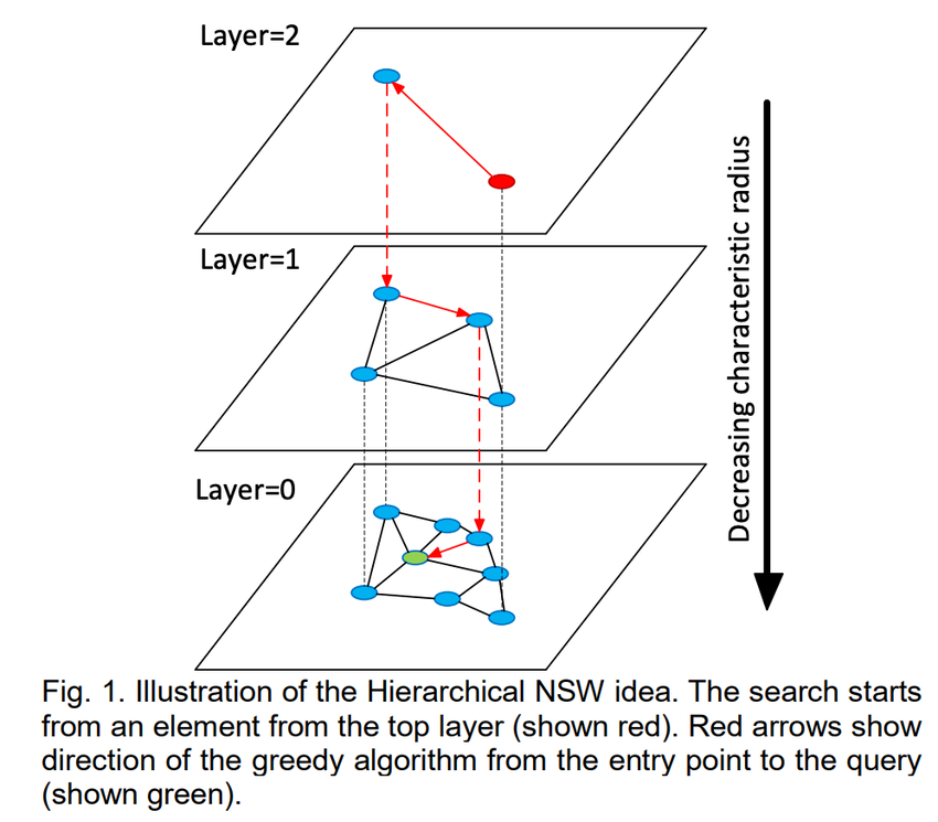
1. The Layered Structure
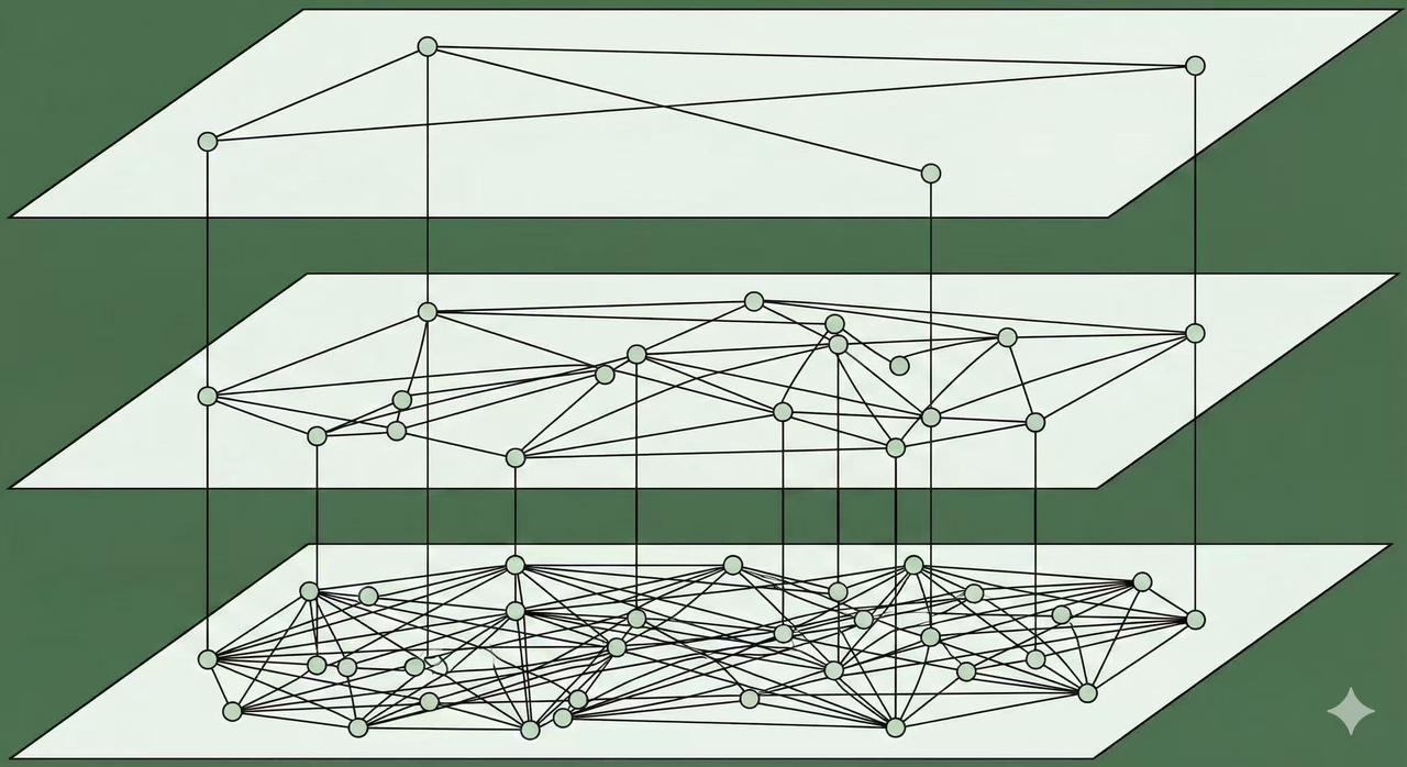
The HNSW index is built as a stack of graphs, from the densest to the sparest top layer:
- Base Layer (
$G_0$): This layer contains all the data points and has the highest density of connections. It is responsible for the final, fine-grained local search. - Top Layers (
$G_1$and above): Each subsequent layer is a sparser subgraph. Nodes in these upper layers establish long-range connections, acting as the "express lanes" for quick, global navigation. The nodes in the top layers are merely a small, randomly selected subset of the nodes in the base layer.
2. Probabilistic Layer Assignment: Building Express Lanes
The assignment of a vector to a specific layer is not deterministic; it is determined by a probabilistic mechanism. This is crucial:
- It ensures that higher layers have exponentially fewer nodes.
- The few nodes that do exist in the top layers are crucial for fast traversal over long distances.
- This randomized structure guarantees that the graph remains robust and well-balanced, avoiding worst-case search scenarios.
3. Search Strategy: Top-Down Greedy Navigation
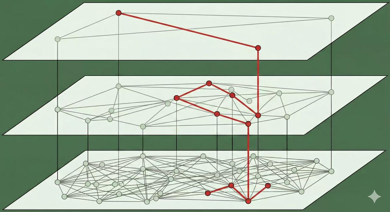
HNSW search is a highly efficient coarse-to-fine process:
- Global Navigation (Upper Layers): Starting from the index's highest layer, the search performs a greedy walk. It uses the sparse, long-range connections to quickly jump across the vector space, moving rapidly toward the general vicinity of the query vector.
- Entry Point Handover: The closest point found in an upper layer is used as the starting point (entry point) for the search in the layer immediately below it.
- Local Refinement (Base Layer $G_0$): Once the search reaches the dense base layer, it is already close to the target. It then switches to a detailed exploration of the local neighborhood, using the many short-range connections to pinpoint the true nearest neighbors.
III. HNSW Compared to Other ANNS Methods
HNSW's power is best understood by contrasting it with two other major categories of ANNS algorithms:
| Category | Algorithm Examples | Underlying Principle | HNSW Advantage |
|---|---|---|---|
| Tree-Based | Annoy (Approximate Nearest Neighbors Oh Yeah) | Builds a series of random projection trees. Average distance across trees determines similarity. | HNSW is generally faster and more accurate. Tree structures suffer more from the curse of dimensionality than graph-based methods. |
| Quantization-Based | Product Quantization (PQ), IVF-PQ | Compresses the high-dimensional vectors into shorter, low-dimensional codes to drastically reduce memory use. | Higher Recall and Speed/Memory Trade-off: Quantization sacrifices recall for extreme memory savings. HNSW offers superior recall, trading speed/accuracy against more memory usage. |
| Other Graph-Based | NSG (Navigable Small World) | A single-layer graph using greedy search. | Solves Local Optima: HNSW's hierarchical structure effectively addresses the issue of greedy search getting stuck in local minima, leading to much higher recall. |
In Summary: HNSW provides the best overall balance between high recall (finding the true nearest neighbors) and high speed (low search latency) in production environments, making it the dominant choice where accuracy is paramount.
IV. Performance Tuning and Conclusion
The performance of an HNSW index is largely controlled by two key parameters, offering a fine-grained trade-off:
$$M$$(Max Connections): Controls the density and robustness of the graph. A larger$M$means more connections, leading to higher accuracy but increased memory consumption and slower index build time.$$E_{f$$(Effective Search Size): Controls the breadth of the search during query time. A larger$E_{f}$means the search explores more candidate neighbors, resulting in significantly higher recall, but at the cost of slower query time.
HNSW is not just an algorithm; it is a dynamic, high-performance indexing method capable of handling massive, high-dimensional data sets with near-logarithmic search complexity. Its robustness and tunable nature have cemented its status as the foundational technology for modern vector databases and large-scale similarity search engines.
V. HNSW And How It Can be Used in VeloDB
VeloDB supports creating ANN Index with HNSW algorithm.
1. Using HNSW In DDL
Approach 1: define an ANN index on a vector column when creating the table. As data is loaded, an ANN index is built for each segment as it is created. The advantage is that once data loading completes, the index is already built and queries can immediately use it for acceleration. The downside is that synchronous index building slows down data ingestion and may cause extra index rebuilds during compaction, leading to some waste of resources.
CREATE TABLE sift_1M (
  id int NOT NULL,
  embedding array<float>  NOT NULL  COMMENT "",
  INDEX ann_index (embedding) USING ANN PROPERTIES(
      "index_type"="hnsw",
      "metric_type"="l2_distance",
      "dim"="128"
  )
) ENGINE=OLAP
DUPLICATE KEY(id) COMMENT "OLAP"
DISTRIBUTED BY HASH(id) BUCKETS 1
PROPERTIES (
  "replication_num" = "1"
);

INSERT INTO sift_1M
SELECT *
FROM S3(
  "uri" = "https://selectdb-customers-tools-bj.oss-cn-beijing.aliyuncs.com/sift_database.tsv",
  "format" = "csv");
2. CREATE/BUILD INDEX
Approach 2: CREATE/BUILD INDEX
CREATE TABLE sift_1M (
  id int NOT NULL,
  embedding array<float>  NOT NULL  COMMENT ""
) ENGINE=OLAP
DUPLICATE KEY(id) COMMENT "OLAP"
DISTRIBUTED BY HASH(id) BUCKETS 1
PROPERTIES (
  "replication_num" = "1"
);

INSERT INTO sift_1M
SELECT *
FROM S3(
  "uri" = "https://selectdb-customers-tools-bj.oss-cn-beijing.aliyuncs.com/sift_database.tsv",
  "format" = "csv");
After data is loaded, you can run CREATE INDEX. At this point the index is defined on the table, but no index is yet built for the existing data.
CREATE INDEX idx_test_ann ON sift_1M (`embedding`) USING ANN PROPERTIES (
  "index_type"="hnsw",
  "metric_type"="l2_distance",
  "dim"="128"
);

SHOW DATA ALL FROM sift_1M

+-----------+-----------+--------------+----------+----------------+---------------+----------------+-----------------+----------------+-----------------+
| TableName | IndexName | ReplicaCount | RowCount | LocalTotalSize | LocalDataSize | LocalIndexSize | RemoteTotalSize | RemoteDataSize | RemoteIndexSize |
+-----------+-----------+--------------+----------+----------------+---------------+----------------+-----------------+----------------+-----------------+
| sift_1M   | sift_1M   | 1            | 1000000  | 170.001 MB     | 170.001 MB    | 0.000          | 0.000           | 0.000          | 0.000           |
|           | Total     | 1            |          | 170.001 MB     | 170.001 MB    | 0.000          | 0.000           | 0.000          | 0.000           |
+-----------+-----------+--------------+----------+----------------+---------------+----------------+-----------------+----------------+-----------------+
2 rows in set (0.01 sec)
Then you can build the index using the BUILD INDEX statement:
BUILD INDEX idx_test_ann ON sift_1M;
BUILD INDEX is executed asynchronously. You can use SHOW BUILD INDEX (in some versions SHOW ALTER) to check the job status.
3. DROP INDEX
You can drop an unsuitable ANN index with ALTER TABLE sift_1M DROP INDEX idx_test_ann. Dropping and recreating indexes is common during hyperparameter tuning, when you need to test different parameter combinations to achieve the desired recall.