


Introduction to Product Quantization
Product Quantization (PQ) is a technique for compressing high-dimensional vectors in order to make large-scale similarity search feasible. In modern AI systems – from image search engines to recommendation systems – data is often represented as high-dimensional vectors (embeddings). Storing and searching through millions or billions of these vectors can be prohibitively expensive in terms of memory and computation. For example, storing 1 billion vectors of 768 dimensions (common for transformer-based embeddings) in full precision can require on the order of 3 terabytes of memory, which is impractical for most applications. PQ addresses this challenge by trading a small amount of accuracy for huge gains in memory efficiency and search speed. Instead of keeping each vector in full detail, PQ compresses vectors into compact codes. This allows systems to fit massive vector datasets in memory and perform approximate nearest neighbor searches much faster. In essence, PQ matters because it enables scalable similarity search– making it possible to search in enormous vector collections (images, texts, user embeddings, etc.) with manageable resource usage and latency.
How Product Quantization Works
At its core, product quantization works by breaking down a vector and quantizing each part independently. This creates a compact representation (a “PQ code”) for each vector and allows efficient distance computations. The process can be understood in a series of steps:
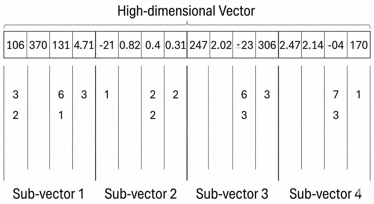
- Subspace Decomposition: Take the original high-dimensional vector and split it into multiple smaller vectors (subvectors). If the original vector has dimensionality
D, we choose a number of segmentsMand divide the vector intoMequal parts of dimensionD/Meach. Each subvector corresponds to a different subspace of the original vector space. For example, a 128-dimensional vector might be divided intoM = 8subvectors of 16 dimensions each. This decomposition is important because it allows us to handle high-dimensional data by dealing with lower-dimensional chunks, which are easier to quantize.
- Codebook Training (Clustering): For each subspace (i.e. for each position out of the
Msegments), we create a codebook of representative vectors. This typically involves running a clustering algorithm (such as K-means) on a large sample of the subvectors for that position. The clustering findsKrepresentative points (centroids) in that subspace. These centroids become the codewords in the codebook for that subspace. Each codebook is essentially a list of prototype vectors that span the subspace. The number of centroidsKis a key parameter – for instanceK = 256centroids per subspace is common, which corresponds to using an 8-bit code for that subvector (since 256 possibilities fit in one byte). The codebook training is done offline (preprocessing) and producesMseparate codebooks (one for each subspace). This step captures the typical patterns in each coordinate chunk of the data.
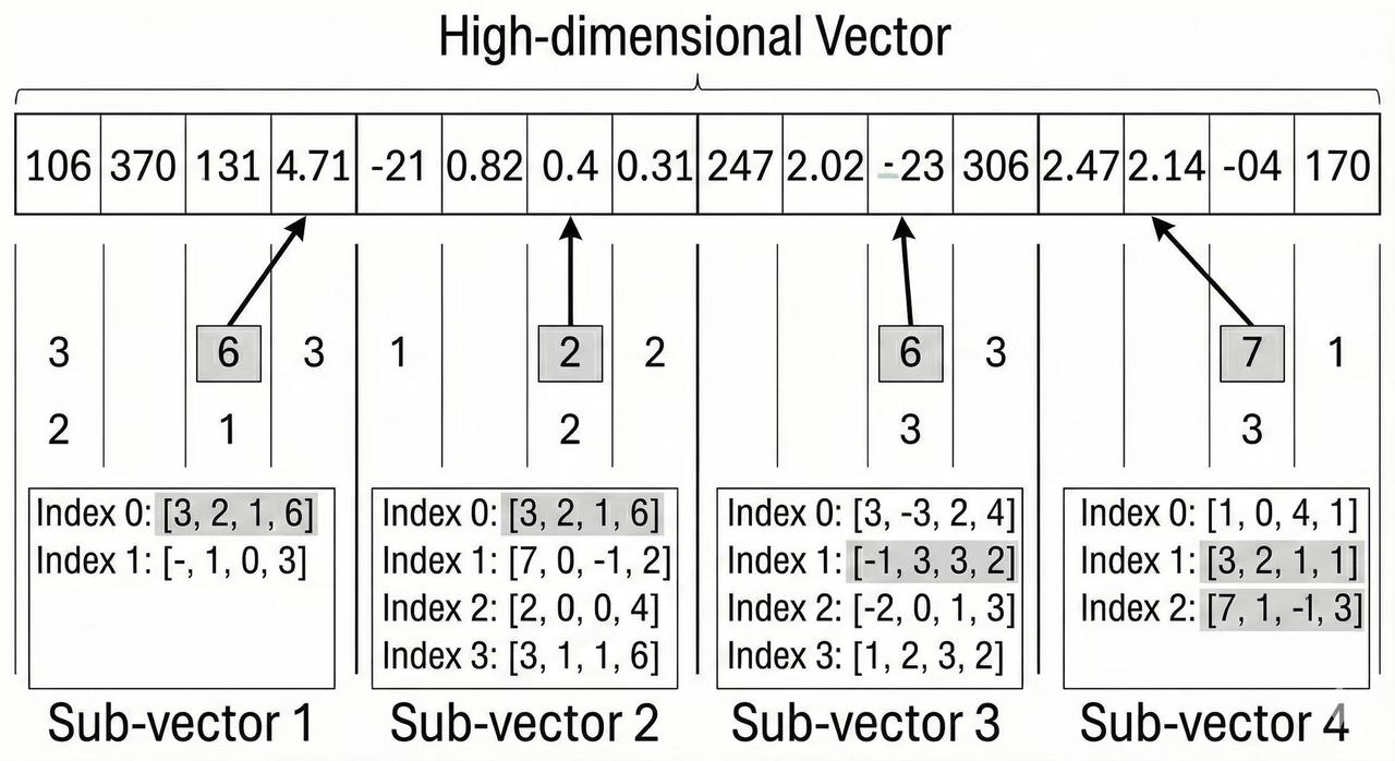
- Encoding Vectors (Quantization): Once we have codebooks, each data vector can be encoded by quantizing each of its subvectors to the nearest centroid in the corresponding subspace codebook. In practice, for a given vector:
- Take the first subvector (the first
D/Mdimensions) and find which centroid in codebook #1 it is closest to. Replace that subvector with the index of the nearest centroid. - Do the same for the second subvector using codebook #2, and so on for all
Msubspaces. After this, instead of storing the full vector of floats, we store an M-length code consisting of centroid indices. This PQ code might look like something as simple as[37, 5, 199, ...](if each number corresponds to the nearest centroid in each subspace). Concatenating these indices yields the compressed representation of the vector. The memory footprint is now justMintegers (often each integer is stored in a byte ifKwas 256, or in a few bits if fewer centroids are used). For example, compressing a 768-dimensional vector withM = 32andK = 256would produce a 32-byte code (versus ~3 KB for the original float vector). This is a drastic reduction in size – the vector is now represented by a handful of bytes. 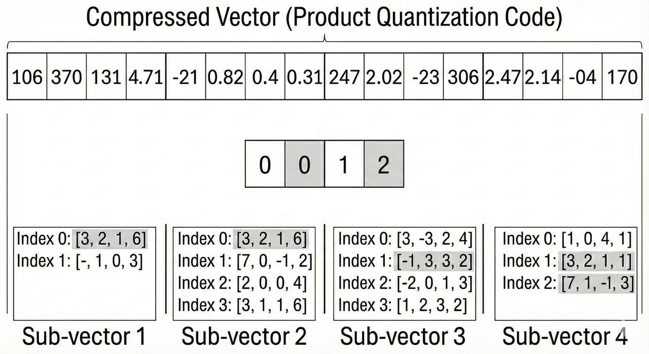
- Take the first subvector (the first
- Decoding and Distance Computation: Given the PQ code for a vector, one can decode an approximate version of the original vector by retrieving each centroid from the codebook and concatenating them. In other words, each index in the PQ code is replaced by the actual centroid vector (the prototype) in that subspace, reconstructing an approximate vector. However, in practice for search, we usually do not need to explicitly reconstruct all vectors. Instead, PQ enables efficient distance computations directly in the compressed domain using the codebooks. The standard approach is known as asymmetric distance computation (ADC). In an ADC setup, when a query comes in (as a full high-dimensional vector), we do not compress the query – instead, we leave the query in its original (full-precision) form. We then compute the distance between the query and each database vector approximately as follows:
- Split the query vector into the same
Msubspaces. - For each subspace
i, for each possible centroid in codebooki, precompute the distance between the query’s subvector and that centroid. (This yieldsMtables of distances, one table per subspace, where each table hasKentries.) - Now, for any database vector’s PQ code, we can compute the distance very fast: we take each subvector index from the code, look up the precomputed distance from the query to that centroid, and sum these distances over all
Msubspaces. This gives an approximate distance between the query and the compressed vector without ever fully decoding the vector or doing high-dimensional math on the fly. Because the heavy computation (distances to centroids) is done for onlyKpossibilities per subspace and then reused, searching through a large database becomes extremely efficient. ADC is “asymmetric” because we compare a full query to compressed vectors (rather than compressing the query as well). This yields more accurate distances than if we also compressed the query (which would be symmetric but compound the quantization error). By using ADC, we leverage the PQ codes to find nearest neighbors with far less computation and memory access than a brute-force scan of full vectors. 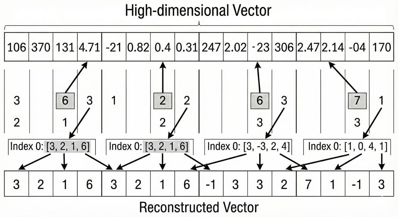
- Split the query vector into the same
Advantages of Product Quantization
PQ offers several significant benefits for handling large-scale vector data:
- Dramatic Compression and Memory Savings: The primary advantage of PQ is the huge reduction in memory footprint. Storing a vector as a short code (often just a few bytes or tens of bytes) instead of hundreds or thousands of bytes means we can keep vastly more vectors in RAM or on faster storage. This compression factor can easily be 20×, 30×, or more while retaining useful information. Such memory savings are crucial when dealing with millions or billions of vectors, making otherwise infeasible datasets manageable.
- Fast Distance Computation and Search Speed: PQ not only compresses data but also accelerates distance calculations. Because computations in PQ largely boil down to table lookups (distance from query subvector to centroid) and summations, the search process can be extremely fast and highly cache-friendly. The small size of PQ codes means more data can fit in CPU caches or GPU memory at once, improving throughput. In practice, querying a PQ-index can be many times faster than scanning full vectors, especially when combined with optimized distance lookup tables and hardware-specific optimizations.
- Scalability to Huge Datasets: Thanks to the memory reduction and speed-ups, PQ allows similarity search systems to scale to very large collections of vectors. It enables billion-scale indexing on commodity hardware or cloud instances by compressing data enough to fit in main memory. The result is that companies can build recommendation engines or semantic search indexes over enormous datasets (images, documents, users) that would otherwise require prohibitive resources. PQ’s efficiency paves the way for scalable AI applications that serve real-time queries on massive data.
- Maintaining Reasonable Accuracy: While PQ is a lossy compression, it is designed to preserve vector distances as much as possible given the code size. When properly tuned, PQ can retain a large portion of the nearest-neighbor structure of the data. This means that, despite heavy compression, the search accuracy (recall of true nearest neighbors) can remain high enough for practical use. In many scenarios, a slight drop in accuracy is acceptable in exchange for huge gains in speed and memory usage. PQ often hits a “sweet spot” where we get significant efficiency improvements with only minor impact on result quality.
Limitations of Product Quantization
Despite its strengths, PQ comes with trade-offs and considerations to keep in mind:
- Quantization Error and Accuracy Loss: By approximating vectors with coarse codewords, PQ inevitably introduces error. The distances computed on PQ codes are approximate, not exact. If the compression is too aggressive (for example, using very few bits or very few subspaces), the reconstructed vectors may be quite far from the originals, leading to missed true neighbors or incorrect nearest-neighbor rankings. In other words, PQ can reduce the recall or precision of a search – some of the actual closest items might not appear in the top results because the distance distortions shuffle the rankings. This accuracy loss is the fundamental trade-off for PQ’s efficiency. Applications that require extremely high recall or exact results may find PQ’s error unacceptable unless paired with refinement steps.
- Sensitivity to Parameters and Data Distribution: The performance of PQ heavily depends on the choice of parameters such as the number of subspaces
Mand the number of centroidsK(or equivalently, the number of bits per subvector). These hyperparameters need to be tuned for the specific dataset and application requirements. For instance, using more subspaces or more centroids per subspace will generally improve accuracy (lower quantization error) but also increase the code size and slow down search somewhat. Conversely, aggressive compression (fewer subspaces or very small codebooks) might degrade accuracy too much. Finding the right balance often requires experimentation. Moreover, PQ assumes that the vector distribution can be effectively factored into independent subspaces – if the data has strong correlations across dimensions or complex structure, the basic PQ (with simple axis-aligned subspaces) might not capture it well. This is one reason techniques like optimized PQ (with rotated subspaces) exist. In short, PQ isn’t one-size-fits-all: it requires careful parameter selection and might work better on some types of data than others. - Training Complexity and Index Build Time: Building a PQ index has a non-trivial upfront cost. The step of training codebooks for each subspace (usually via K-means clustering) can be computationally expensive, especially for very large datasets and high dimensions. For example, if you have many millions of vectors of dimension 768 and you split into 16 subspaces with 256 centroids each, you are effectively running 16 clustering processes on huge amounts of data. This can take significant time and computing resources (CPU or GPU) to get right. Additionally, to train a good quantizer, you need a representative sample of your data; using too small or biased a sample can lead to poor codebooks that hurt search accuracy. Thus, the index construction phase for PQ can be much slower and more complex than for an uncompressed index. Maintaining the index is also more complicated – if new data is added or the data distribution shifts, the codebooks might need retraining or updating (which is not straightforward to do incrementally). This means PQ is best suited for scenarios where you can afford an offline training phase and where the vector dataset is relatively static once indexed.
- Lower Recall Ceilings in Some Cases: Even with ample tuning, a PQ-based search will usually have a ceiling on the recall/accuracy it can achieve for a given code size. If an application demands extremely high recall (nearly exact results), PQ alone might fall short unless the codes are made very long (which diminishes the benefit of using PQ in the first place). In practice, very high accuracy requirements may call for alternative approaches or hybrid strategies (like re-ranking with exact distances). It’s important to recognize that PQ excels when a moderate drop in accuracy is acceptable; it is not intended for scenarios that cannot tolerate any loss of fidelity.
Applications of Product Quantization
PQ has become a standard tool in many large-scale AI and search applications that handle high-dimensional vectors. Some notable areas where PQ is applied include:
- Image and Multimedia Retrieval: In content-based image retrieval and video retrieval systems, images or video frames are often represented by feature vectors (embeddings). Product Quantization was originally popularized in this domain to compress those feature vectors (like SIFT descriptors or deep neural network embeddings) so that huge image databases can be searched quickly for similar content. By using PQ, image search engines can store billions of image feature vectors and compute similarity (e.g. nearest neighbor matches for a query image) much faster, enabling features like finding duplicate/similar images or videos by example.
- Recommendation Systems: Modern recommendation engines rely on high-dimensional embeddings for users and items (products, movies, songs, etc.). Finding similar users or items (or the nearest neighbors to a user’s preference vector) is a common operation for generating recommendations. PQ helps by compressing these large embedding tables, allowing the system to hold more data in memory and search through candidates faster. For example, an e-commerce site with tens of millions of products can use PQ to compress product embeddings, making it feasible to run real-time nearest-neighbor searches to suggest related products or content. The slight loss in accuracy is often acceptable in exchange for being able to scale to all users and items.
- Natural Language and Document Retrieval: In NLP applications like semantic search, question answering, or retrieval-augmented generation, documents or text passages are encoded as embedding vectors. These systems need to retrieve relevant texts given a query vector (often produced by a language model). PQ is widely used to compress and index text embeddings for fast similarity search. It enables, for instance, a question-answering system to scan through a vector index of millions of documents to find those related to a query, all within milliseconds. Without PQ, storing and searching those embeddings would be too slow or memory-intensive. Many AI-driven search services and open-source vector databases for text (used alongside large language models) rely on PQ-based indexes to achieve low latency on large corpora.
- Vector Databases and ANN Services: With the rise of specialized vector database systems and Approximate Nearest Neighbor (ANN) search libraries, PQ has become a built-in option for practitioners. Dedicated vector search engines (both open-source libraries like Faiss and ScaNN, and cloud services or databases like Milvus, Pinecone, and OpenSearch) use product quantization under the hood to handle scale. In these contexts, PQ is one component of the indexing strategy that allows users to store high-dimensional data efficiently and perform queries with configurable speed-accuracy trade-offs. Essentially, any application that needs to serve similarity searches on very large datasets – whether it’s searching through audio embeddings, DNA sequences represented as vectors, or physics simulations – can benefit from the compression provided by PQ. Its versatility and effectiveness have made it a go-to technique in the toolkit for large-scale AI engineering.
Implementations and Engineering Best Practices
Product Quantization has matured to the point where robust implementations and tools are readily available, and there is collective wisdom on how to get the best results. Here we discuss how PQ is used in practice, including libraries, parameter choices, enhancements like OPQ, hybrid indexing strategies, and practical tips for tuning.
Libraries and Tools: The most prominent library for PQ (and ANN search in general) is Facebook AI Research’s Faiss. Faiss provides efficient C++/Python implementations of PQ, optimized for both CPU and GPU. It allows users to create a PQ index (often denoted as IndexPQ or as part of composite indexes) and supports training the quantizers, adding vectors, and performing searches. Many vector database systems and AI frameworks incorporate Faiss or offer similar functionality under the hood. For example, popular vector DBs or search services may expose a setting to enable PQ compression on the stored vectors. Google’s ScaNN is another library that includes quantization techniques for efficient search. Additionally, frameworks like OpenSearch (Amazon’s search service) have introduced support for PQ-based indexes in their k-NN search plugin. In short, engineers typically don’t implement PQ from scratch – they leverage these well-tested libraries. When using them, it’s important to read their documentation on how to train the quantizer and what index types to use (e.g. Faiss has index factory strings to configure combinations like IVF+PQ, etc.).
Typical PQ Parameters: Two key parameters define a PQ setup: the number of subquantizers M (subspaces) and the number of bits per subvector (which determines K, the number of centroids per codebook). A very common choice is to use 8 bits per subvector (256 centroids), as this yields nice byte-aligned codes and a good balance of accuracy vs size. With 8-bit codewords, each subvector’s encoded value is one byte. The value of M is often selected based on the desired code size. For example, if you want each vector to be compressed to 16 bytes, you might choose M = 16 (with 8 bits each, that’s 16 bytes total). If more compression is needed, M could be smaller; for higher accuracy (larger codes), M can be larger (e.g. 32 or 64). In practice, M is typically in the range of 4 to 64. Very large M (creating long codes) might preserve accuracy but then the benefit of compression diminishes and the search slows down because there are more components to sum up for distances. Another consideration is that the vector dimensionality D usually should be divisible by M (so that subvectors are equal in size). If D isn’t divisible, one might slightly adjust M or pad/reduce dimensions (sometimes using techniques like PCA to reduce D to a factorable number). Tuning these parameters involves understanding the memory budget and accuracy requirements: a higher M or more bits gives better recall but uses more memory per vector and possibly longer indexing time. A rule of thumb is to start with something like 8–16 bytes per vector (depending on how large your dataset is and how much accuracy you need) and then adjust if necessary.
Optimized Product Quantization (OPQ): One proven enhancement to standard PQ is Optimized Product Quantization. OPQ addresses the issue that PQ’s effectiveness can be limited if the original feature space isn’t aligned well with the subspaces. In PQ, we naively split the vector by coordinates (e.g. first 16 dimensions as subvector1, next 16 as subvector2, etc.), but these chunks might not capture variance evenly – some chunks might contain highly correlated or high-variance features, while others have low variance, leading to imbalanced quantization error. OPQ introduces a learned rotation (a linear transformation) that is applied to the vectors before splitting into subspaces. In essence, OPQ finds a new coordinate system for the data that spreads out the information more evenly across the M subvectors. It does this by learning a rotation matrix (or a more general orthonormal transform) using the training data, usually aiming to minimize quantization error. After this transform, you proceed with the usual PQ on the rotated data. The result is typically a notable improvement in accuracy for the same code size, because each subvector now carries a balanced portion of the information. OPQ does not add any cost at search time beyond an extra matrix multiplication on the query (and possibly on the data during index build), which is negligible compared to distance computations. Many implementations (Faiss included) support OPQ as an option, and it’s often recommended to use it if you can afford a bit of extra training complexity. In practice, enabling OPQ often yields an immediate boost in recall for a given PQ setting, making PQ competitive with other more complex quantization schemes. It’s an easy win for many use cases.
Hybrid Index Strategies (IVF, HNSW****, etc.): By itself, PQ compresses vectors and speeds up distance calculations, but searching through millions of vectors can still be too slow if you compare a query with every single database vector, even with ADC. That’s why PQ is often combined with a coarser indexing structure that narrows down the search space for each query. A popular strategy is to use an inverted file (IVF) index in conjunction with PQ. This is commonly referred to as an IVF-PQ index. Here’s how it works: an IVF index clusters the full dataset into a large number of partitions (cells) using a separate coarse quantizer (for example, a k-means clustering on full vectors into nlist clusters). Each vector is assigned to its nearest cluster centroid and stored in that bucket (and within the bucket, the vector is stored as a PQ code). At query time, the query is also roughly mapped to a few nearest clusters (using the same cluster centroids), and then you only perform the detailed PQ distance computations on vectors in those selected clusters. This dramatically reduces the number of comparisons per query – you might examine only, say, 1% of the database or even less, depending on how many clusters you probe. The IVF-PQ combination thus achieves two levels of efficiency: coarse filtering by IVF and fast distances by PQ. The trade-off is that IVF introduces another source of approximation (if the query’s nearest neighbor was in a different cluster that you didn’t search, you could miss it). However, by tuning the number of clusters (nlist) and how many clusters are searched (nprobe), one can balance speed vs recall. For instance, increasing nprobe (searching more clusters for each query) will catch more true neighbors at the cost of more computations. In practice, IVF-PQ is one of the most scalable index types and is used in many production systems (it was a key part of Facebook’s billion-scale ANN research). Aside from IVF, other hybrid approaches include using graph-based ANN structures with compression – for example, one could use a HNSW graph where each node’s vector is stored as a PQ code to save memory. This is less common but can be effective: the graph provides fast search and the PQ compresses the data, though one must be careful that the distance approximation doesn’t badly affect the graph traversal. There are also multi-level quantization strategies (like residual quantization or additive quantization) which can be seen as alternatives or complements to PQ, but these tend to be more complex to implement. In summary, combining PQ with a higher-level index is often essential for achieving both speed and scale – PQ takes care of memory and lower-level distance speed, while structures like IVF or HNSW handle the coarse search efficiency.
Practical Tuning Advice: Successfully deploying Product Quantization involves tuning a few knobs and evaluating the results. Here are some practical tips:
- Use a Representative Training Set: The quality of the PQ codebooks is determined during the training phase. Make sure to use a large and representative sample of your vectors when training the subspace centroids. If your data has outliers or multiple distributions (e.g. different categories), ensure the training data covers that variety. Insufficient or non-representative training data can lead to poor compression (high error).
- Tune Code Size vs Accuracy: Determine what code size (bytes per vector) you can afford based on memory limits, then test different configurations around that. For example, if 16 bytes per vector is the target, you might try
M=16, 8 bits(16 bytes) versusM=8, 8 bits(8 bytes, more compression but likely lower recall) versusM=32, 4 bits(16 bytes as well, but using more subspaces with fewer centroids each). Evaluate the recall or error on a validation set for these options. Generally, more bits or more subspaces will increase accuracy but use more memory. Find the lowest code size that still gives acceptable accuracy for your application. - Incorporate OPQ or PCA: If your vectors have some redundant dimensions or highly uneven variance, consider doing a PCA dimensionality reduction or using OPQ’s rotation before quantization. Even reducing the dimension slightly (dropping very low-variance components) can help PQ focus its capacity on the important signal. OPQ is usually a straightforward way to boost performance and is often worth enabling when available.
- Adjust Inverted Index Parameters: If you are using IVF-PQ, the parameters
nlist(number of clusters) andnprobe(clusters searched per query) are critical. A largernlistmeans each cluster (cell) is smaller, which can improve search speed (fewer vectors per cell to scan) but might require searching more cells to not miss good matches. A largernprobeincreases recall at the cost of more work per query. In practice, you might start with something likenlistsuch that each cluster has a few thousand vectors, and then tunenprobeuntil you reach a desired recall level. Keep an eye on the query latency as you do this. - Consider Hybrid Refinement: For applications where accuracy is paramount, a common technique is to use PQ to narrow down candidates, and then re-rank top candidates with the original vectors. For example, you can retrieve the top 1000 neighbors using the PQ-coded distances, then fetch the original vectors for those 1000 and compute exact distances to get the final top 10 results. This “coarse-to-fine” approach lets you benefit from PQ’s speed for most of the work, while preserving accuracy at the end. It does require that you either store the original vectors separately or can compute them on the fly, but often a small re-ranking step is feasible.
- Monitor Quantization Error: It’s useful to quantify how much information loss PQ is causing. You can measure the distortion by reconstructing some sample vectors from their PQ codes and computing an error metric (like the average squared distance between original and reconstructed). If the distortion seems very high for your chosen parameters, you may need to increase codebook size or number of subspaces. Also track the recall of nearest neighbor search versus an exact method to ensure it meets your needs.
- Efficiency Considerations: Implementations like Faiss are quite optimized, but you should still ensure you use them correctly. For instance, after training the PQ index, you typically need to call a
train()method on the index with your training data before adding vectors (this builds the codebooks). When searching, batch your queries if possible to leverage vectorized operations, and prefer computing distances on hardware (Faiss has GPU support for many PQ operations). Also, if using multi-threading, be mindful of memory bandwidth – PQ search is memory-bound in many cases (lots of lookups), so too many threads might saturate it with diminishing returns. - Maintenance and Updates: If your dataset updates frequently (new vectors added over time), note that adding new vectors to a PQ index without retraining is possible, but if the data distribution changes significantly you might eventually need to rebuild the quantizer. Some advanced methods allow dynamic codebook updates, but a simpler approach in engineering practice is to periodically rebuild the index from scratch (or use a fresh sample to train) if you notice degradation in accuracy due to data drift.
By following these practices, engineers can effectively harness Product Quantization to build systems that handle massive vector data efficiently. PQ offers a powerful balance between performance and accuracy, enabling technologies that were otherwise impractical at scale. With the right tuning and hybrid approaches, it continues to be a cornerstone for similarity search in the era of big data and AI.