Inverted File Index (IVF) in Vector Similarity Search

Introduction

The Inverted File Index (IVF) is a widely used data structure for approximate nearest neighbor (ANN) searches in high-dimensional vector spaces. In vector similarity search tasks – such as finding similar images, documents, or user embeddings – an IVF index can dramatically speed up queries compared to brute-force search through all vectors. The core idea of an IVF index is to partition the vector space into clusters (often using an algorithm like k-means) and then restrict searches to only the most relevant clusters. This strategy reduces the search scope and computation, making IVF a popular ANN index for large-scale **vector similarity search **applications. Its design is inspired by the concept of inverted indexes in text search, but instead of mapping words to documents, an IVF index maps cluster identifiers to lists of vectors. The result is an index that balances search speed, accuracy, and memory efficiency, and it has become a backbone of many modern vector databases and libraries (for example, Facebook’s Faiss library).

Architecture and Design of the IVF Index

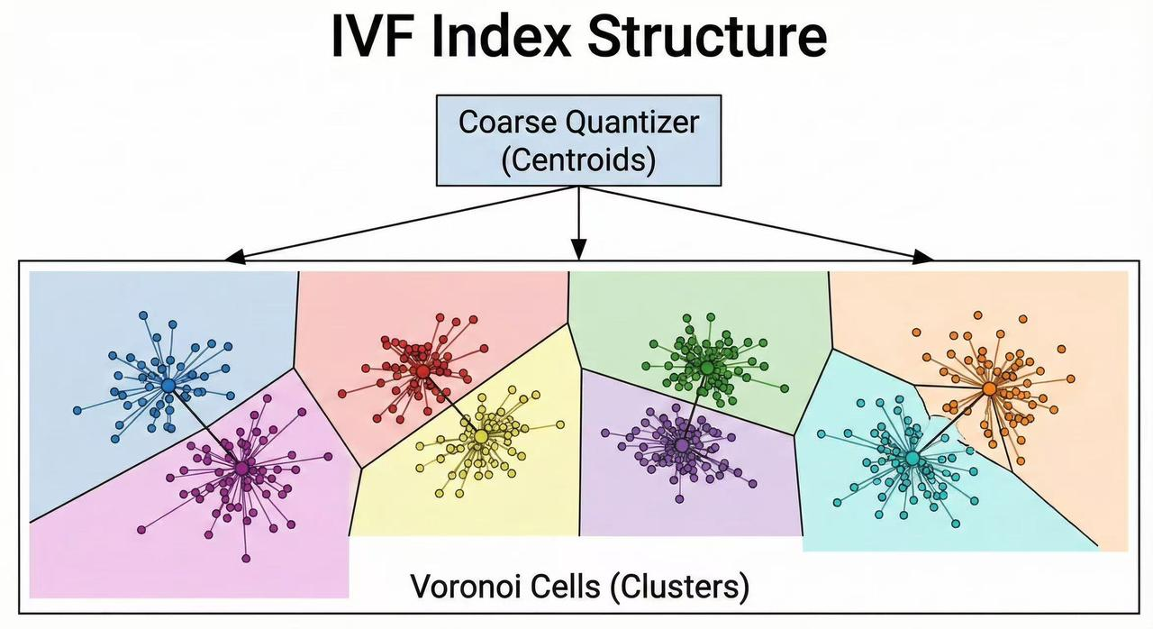
An IVF index is built by organizing vectors into clusters or “cells” and creating an inverted list (posting list) of vectors for each cluster. The process begins with a coarse quantization step: a clustering algorithm (commonly k-means) is applied to the dataset to find a fixed number of cluster centroids. This number is typically denoted as nlist, representing the number of clusters (or inverted lists) in the index. Each centroid is the representative center of a cluster in the vector space.

After computing the centroids, every data vector in the dataset is assigned to its nearest centroid (usually measured by Euclidean distance or cosine similarity). This assignment partitions the whole dataset into nlist groups. For each centroid (cluster), the index stores an inverted list containing the identifiers (and sometimes the vectors) of all data points that belong to that cluster. This data structure is analogous to an inverted index in text retrieval: instead of listing documents for each word, we list vector IDs for each cluster. Organizing the data this way means the index can later retrieve candidates by cluster, rather than scanning all points.

There are different design variations of IVF based on how vectors are stored in these lists:

• IVF Flat (IVFFlat): Each inverted list stores the full, uncompressed vectors that fall into that cluster. This approach retains high accuracy since no information is lost, but reading many full vectors can be memory-intensive and slower if the vectors are high-dimensional.
• IVF with Product Quantization (IVFPQ): Instead of storing full vectors, each vector is compressed into a compact code using Product Quantization (PQ). The inverted lists then contain these PQ codes. During search, distances are approximated using the codes. IVFPQ greatly reduces memory usage and I/O cost, enabling the index to handle billions of vectors with manageable memory. The trade-off is a small loss in precision due to compression. Variants like IVFADC (asymmetric distance computation) refer to using PQ codes for stored vectors while keeping the original query vector uncompressed for distance computations, whereas IVFSDC (symmetric distance computation) compresses both query and database vectors for maximum speed at further cost to accuracy.
• Other Variants: Some implementations integrate IVF with scalar quantization, HNSW graphs, or other secondary structures to improve performance. However, the fundamental architecture remains clustering-based.

Why “Inverted File”? The terminology comes from an analogy to information retrieval: in document search, an inverted file lists documents for each term; in vector search, the IVF index lists vector identifiers for each cluster (which acts like a “term”). This design enables efficient lookups – given a query (like a term or a vector), the system quickly finds relevant lists to scan instead of scanning everything.

Query Execution Pipeline

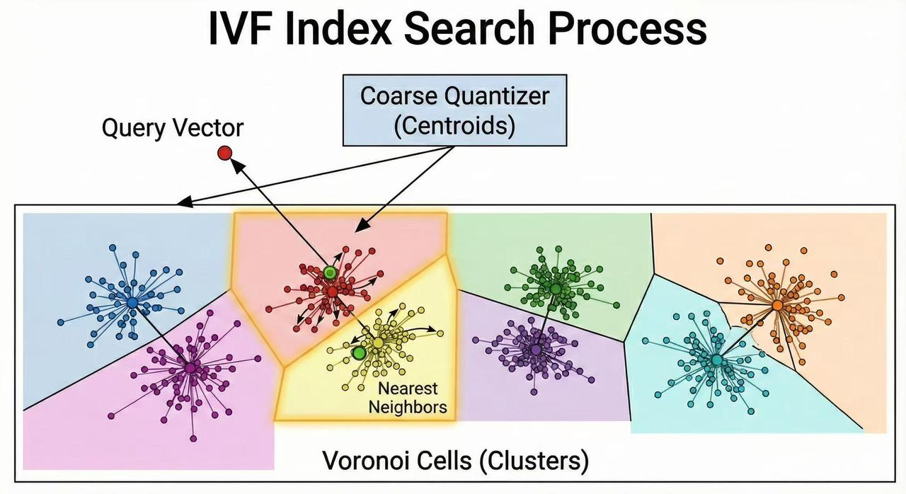
Once the IVF index is built, querying it involves a two-stage search pipeline that dramatically cuts down the work needed for finding nearest neighbors:

1. Coarse Search (Centroid Retrieval): When a query vector is given, the first step is to identify the clusters most likely to contain its nearest neighbors. The query is compared to all cluster centroids (this is a fast operation because the number of centroids nlist is much smaller than the number of data vectors). The index finds the closest centroids to the query and selects the top nprobe centroids. The parameter nprobe controls how many clusters will be searched – effectively how broad the search scope is. For example, if nprobe = 1, the search is confined to the single nearest cluster; if nprobe = 10, the query will examine the 10 closest clusters. Selecting more clusters (higher nprobe) typically increases the chance of finding the true nearest neighbors (higher recall) at the cost of examining more candidates (slower query). This step is akin to finding which “regions” of the vector space the query falls into or near, using the precomputed clustering.
2. Fine Search (Within Selected Clusters): After choosing the most relevant clusters, the search continues by examining only the vectors within those clusters’ inverted lists. The algorithm computes the actual similarity or distance between the query vector and each candidate vector in the selected clusters. If the inverted lists store full vectors (IVFFlat), the exact distance (e.g., Euclidean distance or inner product) is computed. If the lists store compressed codes (IVFPQ or similar), the distance is approximated via those codes (possibly using precomputed lookup tables for efficiency). All candidate distances from the selected clusters are evaluated, and the nearest neighbors overall are identified. Finally, the search returns the top K closest vectors to the query.

This two-stage pipeline significantly improves efficiency by avoiding exhaustive comparison with every database vector. The complexity of a query roughly becomes O(nlist + nprobe * m), where m is the average number of vectors in a cluster, as opposed to O(N) for a brute-force search over N vectors. In practice, with properly chosen parameters, IVF can return high-quality results while examining only a small fraction of the entire dataset.

It’s important to note the role of nlist and nprobe in tuning performance:

• A larger nlist (more clusters) means each cluster is more fine-grained (fewer vectors per cluster). This can lead to faster fine search (because each list is smaller) at the expense of a slightly slower coarse search (more centroids to compare the query against initially) and a requirement for more training data to reliably form many clusters. Extremely large nlist values may also risk creating some empty or sparse clusters if not enough data or if data doesn’t naturally cluster into so many parts.
• A larger nprobe (searching more clusters) increases recall (chances of finding the true nearest neighbors) because it broadens the search to neighboring clusters. However, it also increases the amount of work in the fine search step. In contrast, a very small nprobe (like 1) makes queries very fast but can miss neighbors that lie outside the single closest cluster (the so-called edge problem, where a query near a cluster boundary might actually be closer to points in an adjacent cluster).

By adjusting nlist and nprobe, users can balance speed vs accuracy. A typical strategy is to choose nlist based on the size of the dataset (e.g. sqrt of N or some heuristic) and then adjust nprobe at query time to trade speed for better accuracy as needed. The IVF index’s ability to tune these parameters per use-case is one of its strengths.

Pros and Cons of the IVF Index

Like any indexing strategy, IVF has its advantages and disadvantages. Understanding these helps in deciding when to use IVF and how to configure it for best performance.

Key Advantages:

• High Search Efficiency: IVF greatly accelerates query times by focusing computations on a subset of the data. For large datasets, it can reduce search computations from millions of vectors to just a few thousand or less, with only a minor drop in accuracy.
• Scalability to Large Datasets: The index scales well to very large collections. With proper clustering (and possibly compression), IVF can handle millions or even billions of vectors. The inverted file structure ensures that adding more data mostly increases the number of entries in lists, without a combinatorial explosion in comparisons.
• Memory Efficiency (with Compression): When combined with techniques like Product Quantization (IVFPQ), the memory footprint of the index remains moderate. Storing compressed codes instead of full vectors means you can keep far more items in memory or on disk cache, which is crucial for web-scale search systems.
• Tunable Trade-offs: IVF offers clear tunable parameters (nlist and nprobe) that let practitioners adjust for speed or accuracy requirements. If an application can tolerate slightly lower recall, nprobe can be kept low for lightning-fast responses. If high recall is needed, nprobe can be increased (and perhaps nlist as well) to improve accuracy while still being much faster than brute force.
• Simplicity of Implementation: Compared to some other ANN structures (like complex graph-based indexes), IVF is relatively straightforward. It relies on standard clustering and array data structures (lists of vectors). This simplicity can translate to easier maintenance and understanding. Many find IVF indices easier to debug and reason about than, say, navigating a graph of neighbors.
• Fast Batch and Parallel Searches: Because cluster assignments partition data, searches over different clusters can be parallelized. This makes IVF friendly for batch querying (multiple queries at once) and GPU acceleration. For example, searching 10 clusters for a query could be done by 10 threads or GPU blocks in parallel. This benefit is especially useful for high-throughput systems.

Key Disadvantages:

• Accuracy Dependence on Clustering Quality: The effectiveness of an IVF index heavily depends on how well the initial clustering captures the data distribution. If data points that are true nearest neighbors end up in very different clusters, the index might miss some neighbors unless nprobe is large. Poor clustering (e.g., due to difficult or unfriendly data distributions) leads to lower recall and less benefit from IVF.
• Needs Parameter Tuning: Choosing a good nlist (number of clusters) and nprobe (clusters to search) often requires experimentation and domain knowledge. Too few clusters (small nlist) and the clusters are too broad, offering little speed-up; too many clusters and the query might spend too long checking centroids or suffer from empty clusters. Similarly, nprobe must be set carefully to balance performance vs accuracy. In contrast, some other methods (like certain graph indexes) can often perform well with default settings, whereas IVF typically benefits from tuning to the dataset.
• Dimensionality Challenges: In very high-dimensional spaces, data tends to become more uniformly distributed (the “curse of dimensionality”). This can make meaningful clustering difficult – many points may be almost equidistant or there may not be obvious tight clusters. IVF performance can degrade for such data, as the partitioning may not significantly focus the search. Graph-based methods or other techniques might handle high-dimension relationships more naturally in some cases.
• Static Clustering (Re-training Needs): If the dataset is dynamic (frequently updated with new data or changing in distribution), maintaining an optimal IVF index can be challenging. The initial clustering might become suboptimal as new data arrives that doesn’t fit the original clusters well. While adding new vectors to IVF (assigning them to the nearest existing centroid) is fast, the index may eventually require re-clustering or periodic re-training to ensure search accuracy remains high. This re-training (running k-means again on a growing dataset) can be expensive for very large sets.
• Lower Theoretical Recall Ceiling: Even with large nprobe, if a query’s true nearest neighbor resides in a cluster that is not among the searched ones, IVF will not retrieve it. In contrast, certain graph-based approaches (like HNSW) have a way of navigating to close neighbors even if they start far apart. In practice, IVF can achieve very high recall, but graph methods often edge it out slightly for the last bits of accuracy. Achieving similar recall to exhaustive search might require higher nprobe (slower) or more refined IVF variants (like adding a secondary index).
• Initial Training Cost: Building the IVF index requires clustering the entire dataset (or a large representative sample). Running k-means or other clustering on millions of high-dimensional vectors can be time-consuming and computationally heavy. This is an upfront cost that graph-based indexes or tree-based methods might avoid since they often build incrementally or hierarchically. However, this cost is usually one-time (or occasional for re-training) and is amortized by the faster query performance afterward.

In summary, IVF is a balanced approach offering excellent speedups for ANN search with manageable memory usage, provided the data is amenable to clustering. It does require thought in choosing parameters and maintaining clustering quality, especially as data evolves.

Comparison with Other ANN Indexing Methods

The IVF index is one of several approaches to ANN vector search. It’s helpful to compare it with other popular indexing methods to understand when IVF is the best choice. Below are brief comparisons of IVF with other ANN index structures:

• IVF vs. Brute-Force (Flat Index): A flat index (no index structure, just linear scan) computes distances to every vector for each query. This guarantees 100% accuracy (finding true nearest neighbors) but is prohibitively slow for large datasets. IVF, by contrast, trades a tiny bit of accuracy for a massive gain in speed by only searching a portion of the data. For small datasets or exact search requirements, a flat index can be fine, but for millions of vectors, IVF is far more practical while still retrieving very similar results to exact search in most cases.
• IVF vs. Hierarchical Navigable Small World (HNSW) Graph: HNSW is a graph-based ANN index that organizes vectors in a multi-layer network of neighbor links. It’s known for very high recall and fast search – often HNSW can find nearest neighbors with fewer distance computations than IVF for a given accuracy. Importantly, HNSW tends to handle high-dimensional data and complex distributions well because it doesn’t rely on global clustering; instead, it incrementally builds connections between close points. However, HNSW indexes consume more memory (they store multiple links per vector, which can be large overhead for millions of points) and take longer to construct. HNSW also has its own parameters (like M, efSearch, efConstruction) but generally is less sensitive to tuning than IVF. In practice, if maximum recall and robust performance are required and memory is available, HNSW is often preferred. If memory is limited or data clusters naturally, IVF might be a better fit. IVF is also simpler to implement and can be more straightforwardly parallelized (especially on GPU) since each cluster search is independent, whereas HNSW’s graph traversal is harder to batch efficiently.
• IVF vs. Tree-Based Indexes (e.g., KD-Trees, Ball Trees, Annoy): Tree structures partition data recursively (like building a binary space partition or multiple random projection trees). They work well for moderate dimensions and can give good speed-ups for smaller datasets. However, in high-dimensional spaces (e.g., hundreds of dimensions), tree-based methods suffer as the partitioning becomes less effective (many branches must be explored). IVF’s flat clustering can sometimes outperform trees in high dimensions because it doesn’t require as strict a hierarchy; it just groups points in a single level of clusters. Annoy (which builds multiple random trees) and other tree-based ANN methods are competitive up to a point, but beyond a certain data size and dimensionality, IVF and HNSW usually outperform them. Trees also can be memory-light (just storing split boundaries) and have fast build times, but their recall at high precision might be lower than IVF or HNSW for large, complex datasets.
• IVF vs. Locality-Sensitive Hashing (LSH): LSH uses random projection hash functions to bucket vectors such that similar vectors fall into the same buckets with high probability. Like IVF, LSH limits comparisons to vectors in the same bucket as the query’s hash. LSH doesn’t require a training phase like clustering, and it’s relatively easy to implement. However, to achieve high recall, LSH often needs many hash tables or long hash codes, which increases memory and query time (multiple lookups). LSH performance also deteriorates as dimensionality grows, because random projections become less discriminative. In contrast, IVF explicitly learns data-driven clusters which can capture data distribution better than random hashing. As a result, IVF tends to achieve a better speed-accuracy trade-off than basic LSH for many high-dimensional tasks. Modern ANN systems seldom use pure LSH if alternatives like IVF or HNSW are available, except in special cases or as part of hybrid solutions.
• IVF vs. Product Quantization (PQ) alone: Product Quantization was mentioned earlier as a compression technique and sometimes considered an ANN approach by itself (e.g., one could do an exhaustive search on compressed codes, which is faster than on full vectors). PQ alone (without IVF) can accelerate searches by using codebooks to estimate distances quickly, but it still has to scan through all data points’ codes unless combined with another structure. IVF and PQ are actually complementary: IVF reduces the number of candidates via clustering, and PQ speeds up the distance computations and reduces memory usage. Together (IVFPQ), they form a powerful compound index: IVF narrows down where to search, and PQ makes the how to search faster and more memory-efficient. Comparatively, an HNSW index can also use compression (like storing vectors as PQ codes on nodes), but IVF+PQ has been a classic solution for web-scale vector search (for example, in Facebook’s original billion-scale image search paper using IVFPQ). So it’s often not IVF vs PQ, but rather IVF with PQ versus other methods.

In summary, IVF indexes excel in scenarios where the data can be effectively clustered and memory is a concern, or when one needs an index that is simple and scalable. Graph-based indexes like HNSW often win on pure recall and sometimes speed, but require more memory. LSH and trees are more niche nowadays, with trees being good for lower dimensions and LSH being useful for certain theoretical guarantees or small-scale applications. A common strategy in industry is to try IVF (possibly with PQ) first for very large datasets, and if recall is insufficient, consider switching to or combining with an HNSW index. In many vector database systems, you actually have the option to choose or even stack these methods (for instance, IVF-HNSW hybrid indexes exist, where IVF does coarse clustering and HNSW graphs index within each cluster). The choice depends on the specific requirements of accuracy, latency, memory, and the nature of the data.

Real-World Implementation: FAISS IVF Example

One of the most popular libraries for vector similarity search is Facebook’s Faiss (Facebook AI Similarity Search), which provides efficient C++/Python implementations of many ANN indexes, including IVF. Faiss makes it straightforward to build and use an IVF index. Let’s walk through a simple example of creating an IVF index in Faiss and performing a query, to illustrate the concepts described above:

import faiss
import numpy as np

# Suppose we have a dataset of N vectors, each of dimension d
d = 128                            # dimensionality of vectors
nb = 1000000                       # number of database vectors (1 million for example)
nlist = 1000                       # number of clusters (centroids) for IVF
nprobe = 10                        # number of clusters to search at query time

# Prepare some random data as an example (in practice, use real vectors)
np.random.seed(0)
data_vectors = np.random.rand(nb, d).astype('float32')

# 1. Define the coarse quantizer (centroid index) - using a flat (brute-force) index for centroids
#    Here IndexFlatL2 means an index that computes L2 distances for clustering.
quantizer = faiss.IndexFlatL2(d) 

# 2. Create the IVF index, with the quantizer, dimension, and number of clusters (nlist)
index = faiss.IndexIVFFlat(quantizer, d, nlist, faiss.METRIC_L2)

# 3. Training the IVF index - this runs the clustering (k-means) on a sample of the data
index.train(data_vectors)   # Faiss needs the index to be trained before adding vectors

# 4. Add data vectors to the index - they will be assigned to the nearest centroids
index.add(data_vectors)

# (Optional) You can also add vectors in smaller batches or one by one as data comes in.

# 5. Perform a search query
query_vector = np.random.rand(1, d).astype('float32')  # a single query vector
index.nprobe = nprobe    # set how many clusters to search
distances, indices = index.search(query_vector, k=5)   # find 5 nearest neighbors

print("Nearest neighbor indices:", indices)
print("Distances:", distances)

In the above code:

• We use IndexFlatL2 as the quantizer. This is a simple index that allows computing L2 distances between the query and each centroid. The quantizer is responsible for mapping the query to the closest centroids. (Faiss also supports other quantizers, like IndexFlatIP for inner product, or one can even use a trained PCA or other structures as quantizer, but a flat L2 index is common for IVF.)
• We create an IndexIVFFlat which is an IVF index storing full vectors in each inverted list (Flat means no compression on the vectors). We specify nlist (the number of clusters). The metric is set to L2 (Euclidean) in this case.
• We call index.train(data) to perform clustering. Under the hood, Faiss will take a sample of the data (or all of it if not too large) and run k-means to find nlist centroids. If the index isn’t trained, you cannot add vectors to it yet.
• After training, we add the dataset vectors to the index with index.add(). Faiss will assign each vector to its nearest centroid and store it in the corresponding inverted list.
• At query time, we set index.nprobe = 10 (for example) to search the 10 closest clusters to the query. The search function then finds the top 5 nearest neighbors to our query vector within those clusters. It returns both the distances and the indices (identifiers) of the nearest vectors.

Faiss provides many variations of IVF; for instance, IndexIVFPQ to use Product Quantization for storing vectors (trading accuracy for memory and speed), or IndexIVFSpectralHash for other types of compression, etc. There’s also an IndexIVFScalarQuantizer. In practice, one might choose IndexIVFPQ when dealing with extremely large datasets to keep memory usage low. Building an IVFPQ index in Faiss is similar: you would specify the number of PQ segments (subvector clusters) in addition to nlist, and Faiss will train both the coarse quantizer and the product quantizer codebooks.

Performance in Practice: In real-world applications, Faiss IVF indexes can achieve very high throughput and low query latencies. For example, an IVF index with a million vectors and a good choice of nlist can answer queries in a few milliseconds on a CPU, and even faster on a GPU. By adjusting nprobe, you can often reach ~90-95% of the recall of an exact search while being orders of magnitude faster. This makes IVF indexes extremely useful for tasks like image similarity, approximate search in recommendation systems, or as a backend for semantic search in NLP, where slight approximations are acceptable.

Modern vector search systems often allow using IVF in combination with other techniques. As mentioned earlier, one common approach is IVF+PQ for compressing vectors. Another approach is to use IVF with reranking: first use IVF to get a candidate list quickly, then re-compute exact distances on those candidates (possibly using the original data or a secondary index) to improve accuracy – this still saves time by not rechecking all points, just those shortlisted by IVF.

In summary, the Inverted File Index remains a fundamental component in the ANN index toolkit. Its clustered approach to vector similarity search provides a compelling balance of speed, scalability, and acceptable accuracy. FAISS IVF implementations have demonstrated that this method can scale to billions of vectors and still return results with low latency. While newer methods like HNSW graphs compete closely, IVF’s simplicity and efficiency (especially when paired with quantization) ensure that it continues to be a go-to solution in many real-world vector search engines and libraries.

IVF in VeloDB

VeloDB supports HNSW vector indexes, and it also provides an IVF (Inverted File Index) implementation. Using IVF in VeloDB is almost identical to using HNSW — you simply change the index_type to IVF and configure the relevant parameters such as nlist and nprobe.

Below is a minimal example showing how to use IVF in VeloDB.

1. Creating a Table with an IVF Vector Index

CREATE TABLE example_ivf_vector_table (
    id INT,
    embedding ARRAY<FLOAT> NOT NULL,
    INDEX idx_emb (`embedding`) USING ANN PROPERTIES(
        "index_type"="ivf",
        "metric_type"="l2_distance",
        "nlist"="1024",
        "dim"="128"))
ENGINE=OLAP
DUPLICATE KEY(id)
DISTRIBUTED BY HASH(id) BUCKETS 5
PROPERTIES (
    "replication_allocation" = "tag.location.default: 1"
);

2. Inserting Data

INSERT INTO example_ivf_vector_table VALUES
(1, [0.1,0.2,...]),
(2, [0.4,0.3,...]),
...

3. Running a Vector Search

SELECT id,
       l2_distance_approximate(embedding, [0.12, 0.19, ...]) AS dist
FROM example_ivf_vector_table
ORDER BY dist
LIMIT 10;