


Chapter 1: Introduction—The Search Dilemma in High-Dimensional Space
1.1 The Rise of Vector Embeddings and the Curse of Dimensionality
The rapid advancement of deep learning, particularly Large Language Models (LLMs), has driven a fundamental shift in data representation. Complex data like text, images, and audio are now encoded as high-dimensional, dense vectors (Vector Embeddings). These embeddings capture the intrinsic semantic meaning and relationships within the data.
However, this powerful representation introduces a significant computational hurdle: the Curse of Dimensionality. As the number of dimensions (d) grows, the data space becomes exceedingly sparse. Traditional spatial indexing methods, which scale exponentially with dimension d, become computationally infeasible for the massive, high-dimensional datasets prevalent in industrial applications, often containing billions of vectors. An efficient similarity retrieval mechanism is therefore essential.
1.2 The Limitation and Cost of Exact Nearest Neighbor (ENN)
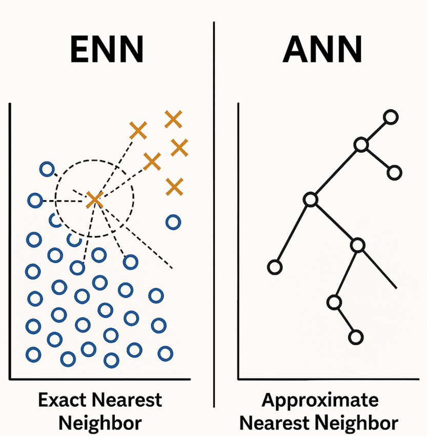
Exact Nearest Neighbor (ENN or NN) search aims to find the k data points in the dataset that are mathematically closest to a given query point. While ENN offers the highest possible accuracy (100% recall), its implementation typically relies on Exhaustive Search, requiring the query vector to be compared against every vector in the dataset.
The query time complexity of this approach is linear, O(N⋅d), where N is the dataset size and d is the dimension. For industrial datasets with billions of vectors (N∼109) and hundreds of dimensions, this linear complexity is computationally prohibitive, resulting in excessive latency and resource consumption. This makes ENN unsuitable for high-throughput, low-latency applications.
1.3 The Core Value of ANN: Trading Precision for Speed
Approximate Nearest Neighbor (ANN) search is the pragmatic solution developed to overcome the computational bottleneck of ENN. ANN algorithms are designed to find a data point that is very close to the query point, even if it is not guaranteed to be the absolute closest one.
This strategy sacrifices a minute, often tolerable, amount of precision (recall) in exchange for massive improvements in speed and performance. ANN achieves this by employing intelligent shortcuts and complex data structures (such as hierarchical graphs, hash buckets, or partitioned clusters) to navigate the high-dimensional space efficiently. It reduces the search complexity from linear O(N⋅d) to sub-linear, enabling millisecond-level queries on billion-scale datasets.
ANN is a practical compromise that effectively mitigates the Curse of Dimensionality.
ANN and ENN Comparison
| Feature | Exact Nearest Neighbor (ENN) | Approximate Nearest Neighbor (ANN) |
|---|---|---|
| Objective | Find the ABSOLUTE closest k vectors (100% Recall) | Find VERY CLOSE k vectors (Acceptable Recall, e.g., 98%) |
| Query Complexity | Linear O(N⋅d) | Sub-linear |
| Speed | Slow (High Latency) | Fast (Low Latency) |
| Resource Usage | High (Time and Memory) | Low |
| Applicability | Small, low-dimensional datasets | Large-scale, high-dimensional (industrial grade) |
Schematic Illustration of Approximate Nearest Neighbor (ANN)
This diagram illustrates the fundamental process and trade-off of the Approximate Nearest Neighbor approach.
| Component | Exact Nearest Neighbor (ENN) | Approximate Nearest Neighbor (ANN) |
|---|---|---|
| Objective | Find the ABSOLUTE closest K vectors (100% Recall) | Find VERY CLOSE K vectors (High Recall, e.g., 98%) |
| Search Space | Entire Dataset (N vectors) | Restricted Subset (N_probe clusters/nodes) |
| Search Path | Linear / Brute-Force Check | Optimized Data Structure (HNSW Graph, IVF Clusters) |
| Result | Guaranteed Best Match (Highest Accuracy) | High Speed / Low Latency (Sacrifices tiny precision) |
Conceptual Flow:
Chapter 2: Performance Metrics and Engineering Trade-offs
The successful deployment of an ANN system requires careful evaluation and trade-off of several key performance indicators (KPIs), as the algorithm choice and parameter configuration directly impact usability and economics.
2.1 Similarity Metrics and Distance Functions
ANN algorithms rely on a distance metric or similarity metric to define "closeness." Common metrics include:
- Euclidean Distance (L2): The most straightforward geometric distance, measuring the straight-line separation between two vectors.
- Cosine Similarity: Measures the angle between two vectors, often used for semantic similarity as it is independent of vector length. It is widely used in Natural Language Processing (NLP) embeddings.
- Dot Product (Inner Product): Used in contexts where both the magnitude and direction contribute to similarity. Specialized algorithms, such as Google's ScaNN, are optimized for high-accuracy inner-product search.
2.2 Core Performance Evaluation Metrics
Four key metrics are typically used to assess the utility of an ANN system:
- Recall@k: The primary measure of search quality. It calculates the proportion of the k nearest neighbors found by the ANN algorithm that are members of the exact nearest neighbor (ground truth) set. Engineering practice often targets Recall@10 or Recall@100.
- Queries per Second (QPS): Measures the throughput—the number of queries the system can handle per second—reflecting speed and capacity.
- Latency: The response time for a single request, often measured as Mean Latency or P99 Latency (the latency that 99% of requests fall below). Low P99 latency is critical for user-facing, real-time applications.
- Index Import Time: The total time required to build the ANN index. This metric is important for large-scale scenarios requiring frequent updates or rapid deployment.
2.3 The Recall vs. QPS Engineering Trade-off
ANN performance tuning is fundamentally a multi-objective optimization problem, centered on the inverse relationship between recall and throughput (QPS).
Generally, increasing algorithm configuration settings to boost recall requires more computational work and time, leading to a drop in QPS, and vice-versa. For instance, in the HNSW algorithm, increasing the efSearch parameter improves recall by enlarging the candidate list during the query but decreases QPS.
System designers must determine a minimum acceptable recall threshold based on the application's Service Level Objectives (SLOs) and then maximize QPS at or above that threshold. For example, a Retrieval-Augmented Generation (RAG) system demands extremely high recall to prevent missing information or generating "hallucinations," thus prioritizing recall over maximum QPS.
For evaluating hardware efficiency, architects look at the QPS/vCore metric, which indicates the throughput achievable per single CPU core. This is crucial for assessing scalability and the Total Cost of Ownership (TCO) in cloud deployments.
Chapter 3: The ANN Algorithm Landscape: Four Major Families
The field of ANN search has developed diverse algorithmic strategies to achieve scalable, high-speed querying. These algorithms are typically classified into four main families based on their underlying data structure and optimization strategy.
3.1 Classification of ANN Algorithms
- Graph-based Methods: These algorithms construct a graph connecting data points and use graph traversal mechanisms, often based on the "Small-World Network" principle, to quickly locate neighbors in a few steps. Key algorithms include Hierarchical Navigable Small World (HNSW) and SSD-optimized DiskANN.
- Quantization and Clustering Methods: These accelerate search by either partitioning the vector space using clustering (e.g., Inverted File, IVF) to narrow the search scope, or by compressing the vectors using quantization (e.g., Product Quantization, PQ) to reduce memory usage and distance computation cost. Representative algorithms are IVF-PQ and ScaNN.
- Hash-based Methods: Represented by Locality-Sensitive Hashing (LSH), these methods design hash functions that ensure similar vectors have a high probability of being mapped to the same hash bucket, allowing for fast filtering of dissimilar vectors via hash lookups.
- Tree-based Methods: These algorithms recursively partition the data space to construct a hierarchical tree structure. Search is confined to a specific leaf node or region associated with the query point through tree traversal. Examples include KD-Tree and Annoy (based on Random Projection Trees).
3.2 Algorithm Selection and Comparison
The choice of ANN algorithm depends on the application's specific needs regarding dataset size, data dynamism, hardware constraints, and precision requirements. The modern trend often focuses on HNSW (speed and recall) and IVF-PQ (scale and memory efficiency).
| Algorithm Family | Representative Algorithms | Core Innovation | Search Complexity | Applicable Scenarios |
|---|---|---|---|---|
| Graph | HNSW, DiskANN | Hierarchical connections, Small-World Network | Efficient Sub-linear | High recall, real-time search, dynamic data |
| Quantization/Clustering | IVF-PQ, ScaNN | Coarse filtering and vector compression | High throughput, low memory | Billion-scale, memory-constrained |
| Hash | LSH | Locality-sensitive functions | Fast filtering | Streaming data, theoretical guarantees, large-scale duplicate detection |
| Tree | Annoy | Random projection trees (RPT) | Memory mapping, lightweight deployment | Static data, moderate scale, simplicity |
Chapter 4: Graph-based Methods: Deep Dive into HNSW
Hierarchical Navigable Small World (HNSW) is currently one of the most prevalent and high-performing ANN algorithms in industrial use, known for its high recall and efficient real-time performance.
4.1 HNSW Structure: Hierarchical Navigation
HNSW is inspired by Navigable Small-World Networks and Skip Lists, building a multi-layered graph structure.
- Hierarchical Layers: The HNSW index consists of multiple graph layers, each representing a different level of abstraction of the dataset.
- Top Layers (Abstraction): Contain the fewest nodes, acting as entry points for search. They feature "long-range" edges for rapid, coarse navigation across the data space, which is key to the small-world property.
- Base Layer (Detail): Contains all data points, with the shortest edges used for the final, fine-grained search.
- Search Efficiency: This structure allows a query to start at the top layer, quickly zoom into the target neighborhood, and then progressively descend to the lower layers, refining the search area until the k nearest neighbors are found without exhaustive search.
4.2 HNSW Query Process and Parameter Control
The HNSW query process is an iterative greedy search that navigates down the hierarchy. Starting from an entry point in the highest layer, the search follows the path closest to the query vector (q), descends to the next layer, and continues refining the search until the base layer is reached.
The performance (the recall vs. QPS trade-off) of HNSW is directly controlled by three key parameters:
| Parameter | Description | Effect of Increasing Value (Positive) | Cost of Increasing Value (Negative) |
|---|---|---|---|
| M | Max connections per node | Better recall | Larger index size, longer index time |
| efConstruction | Search depth during index building | Higher quality graph, better future recall | Longer index time, higher computational cost |
| efSearch | Search depth during querying (Candidate list size) | Better recall | Increased query latency, lower QPS |
The efConstruction parameter determines the quality of the graph and thus the potential for future query performance, while efSearch directly controls the computation required during the query itself. Increasing efConstruction significantly improves future recall but sacrifices index construction time. This fine control makes HNSW the preferred choice for complex applications like RAG that require very high recall.
Chapter 5: Quantization and Clustering Methods: IVF-PQ
For massive datasets reaching billions of vectors where memory resources are limited, purely graph-based methods can be constrained by memory consumption. IVF-PQ (Inverted File with Product Quantization) is a hybrid strategy designed specifically to address the storage and search efficiency of very large datasets by combining space partitioning and vector compression.
5.1 Coarse Filtering: Inverted File (IVF)
The Inverted File (IVF) index handles coarse-grained filtering:
- Space Partitioning: IVF first performs a coarse clustering (typically k-means) on the entire dataset into Nlist clusters (centroids). Each vector is assigned to its nearest centroid, partitioning the space into inverted lists.
- Search Acceleration: When a query vector q is received, the algorithm compares q only against the centroids, selecting only the Nprobe closest clusters (inverted lists) for detailed search. This pre-filtering mechanism drastically shrinks the search space from N to Nprobe, greatly boosting query speed.
5.2 Vector Compression: Product Quantization (PQ)
Product Quantization (PQ) is primarily motivated by the need to drastically reduce the memory cost of storing high-dimensional vectors.
- Vector Segmentation: PQ splits an original D-dimensional vector into m non-overlapping, equally sized subvectors.
- Sub-codebook Generation: Each subvector space is independently clustered to generate a sub-codebook. The subvector is then replaced by the ID of its nearest sub-centroid.
- Encoding and Compression: The final compressed vector representation consists of m sub-centroid IDs. This technique can achieve up to 97% memory compression, making the storage of billions of vectors feasible.
- Distance Calculation: During query time, PQ uses the encoded representation and pre-computed distance tables to quickly approximate the distance, further accelerating the search.
5.3 Hybrid Indexing: IVF-PQ
IVF-PQ combines Inverted File and Product Quantization. IVF handles the coarse-grained partitioning and search range reduction, while PQ manages the fine-grained search and data compression within the selected clusters. This hybrid approach optimizes both speed and memory efficiency, achieving total search speed increases of over 90 times compared to non-quantized indexes. This makes IVF-PQ an excellent solution for "billion-scale, memory-constrained" datasets.
More advanced techniques, such as Google's ScaNN, use "anisotropic" vector quantization to learn and minimize quantization error, offering higher precision compared to the standard "isotropic" PQ approach by aligning quantization regions with the actual data distribution.
Chapter 6: Hashing and Tree-based Methods: LSH and Annoy
Hash-based and tree-based methods offer alternative architectures for ANN search.
6.1 Locality-Sensitive Hashing (LSH): Principle
Locality-Sensitive Hashing (LSH) is a probability-based technique for dimensionality reduction and retrieval.
- Core Idea: LSH designs a family of hash functions H with the property of locality sensitivity: similar data points in the original space (close distance) have a high probability of being mapped to the same hash bucket (collision); dissimilar points have a low collision probability.
- Search Process: By using LSH, a query point q only needs to compute its hash value and search the small subset of candidate vectors within the corresponding hash bucket, avoiding the exhaustive comparison against the entire dataset.
- Implementation: LSH often uses random projection techniques for dimension reduction. Examples include MinHash (for Jaccard similarity in document deduplication) and SimHash (using random hyperplane projections to approximate Cosine distance).
- Trade-offs: LSH provides strong theoretical guarantees and is highly suitable for streaming data. However, achieving high recall in very high dimensions may require a large number of hash functions and tables, potentially making it less memory and performance efficient than HNSW or IVF-PQ in certain industrial settings.
6.2 Tree-based Methods: Annoy and Random Projection Trees (RPT)
Annoy (Approximate Nearest Neighbors Oh Yeah), developed by Spotify, is a lightweight ANN library that primarily uses Random Projection Trees (RPT).
- RPT Principle: Annoy builds multiple independent Random Projection Trees to partition the vector space. During construction, the data is recursively split by a randomly generated hyperplane until the desired leaf node size is reached. RPT is effective at handling high-dimensional data while preserving the relative distances between points.
- Multi-Tree Robustness: Annoy's key feature is the construction of multiple independent trees (ntrees). Each tree offers a different perspective on the data space partitioning. Querying simultaneously traverses multiple trees and merges the results, which significantly improves recall robustness by reducing the chance of missing a neighbor due to a poor split in a single tree.
- Engineering Advantages: Annoy is designed for simplicity and memory efficiency, utilizing memory-mapped files for low memory usage and fast loading. However, once built, the Annoy index is typically read-only, which limits its application in scenarios requiring frequent real-time data updates. It is ideal for static datasets and read-intensive recommendation systems.
Chapter 7: Engineering Practices and Ecosystem Comparison
The true value of ANN algorithms lies in their industrial implementations, packaged in mature libraries and vector databases, each optimized for different hardware and application needs.
7.1 Overview of Industrial ANN Libraries
- FAISS (Facebook AI Similarity Search): Developed by Meta, this open-source library specializes in efficient similarity search and clustering of dense vectors. It is renowned for its extensive support for quantization methods (like IVF-PQ) and powerful GPU acceleration, making it the preferred choice for billion-scale and computationally intensive tasks.
- Annoy: Developed by Spotify, it emphasizes lightweight deployment and simplicity. Its RPT-based architecture excels in memory-mapped file usage and static datasets.
- ScaNN (Scalable Nearest Neighbors): Developed by Google, it is optimized for high-accuracy search for inner-product similarity. It uses learned methods, such as anisotropic quantization, and achieves high efficiency on TPU/GPU platforms.
7.2 Library Selection and Deployment Considerations
The choice of ANN library depends on the system's core business objectives:
- For Maximum Throughput and Scale: Choose FAISS, leveraging its GPU acceleration and quantization techniques for high QPS on massive data.
- For High Precision (especially Inner-Product): Choose ScaNN, which is algorithmically designed for high-accuracy retrieval.
- For Simplicity and Memory Efficiency: Choose Annoy, suitable for resource-limited or static data environments.
- For High Recall and Incremental Updates: Choose HNSWlib or HNSW-based vector databases, as HNSW natively supports efficient incremental updates for real-time data streams.
Pure ANN libraries are increasingly evolving into full-featured vector databases that integrate high-performance ANN algorithms (like HNSW) with enterprise features such as ACID compliance, disaster recovery, data security, and governance, and complex querying capabilities (e.g., Filtered ANN Search, FANNS).
| Library Name | Core Algorithm Type | Primary Optimization Goal | GPU Support | Dynamic Data Support | Typical Application |
|---|---|---|---|---|---|
| FAISS (Meta) | Quantization/IVF/Graph | Large-scale, high throughput, GPU acceleration | Strong | Weaker (Prefers static data) | Image/video retrieval, large-scale clustering |
| Annoy (Spotify) | Tree (RPT) | Simple deployment, memory efficiency | No | Poor (Read-only/Static) | Static recommendation systems, lightweight deployment |
| ScaNN (Google) | Learned Quantization | Extreme accuracy, Inner-product similarity | Yes (TPU/GPU) | Strong | LLM applications, high-precision recommendation |
| HNSWlib/Milvus | Graph (HNSW) | High recall, real-time updates | Varies by wrapper | Good (Incremental updates) | Real-time vector databases |
Chapter 8: ANN Applications in Modern AI Systems
ANN technology is the cornerstone of modern AI infrastructure, enabling efficient semantic matching and knowledge retrieval.
8.1 Semantic Search and Recommendation Systems
ANN has significantly advanced information retrieval and e-commerce:
- Semantic Search**:** By encoding queries and documents into vectors, ANN enables search based on semantic intent rather than traditional keyword matching. This capability allows search engines to handle complex, context-aware queries.
- Recommendation Systems: In streaming services or e-commerce platforms, ANN quickly compares user preference vectors with vast item vectors. It efficiently retrieves highly relevant approximate matches even if they are not exact, facilitating real-time, high-relevance content or product recommendations. ANN can achieve search speeds on billions of documents within milliseconds.
8.2 ANN's Central Role in RAG (Retrieval-Augmented Generation)
Retrieval-Augmented Generation (RAG) models solve the knowledge currency and "hallucination" problems of Large Language Models (LLMs) by grounding generation in external information. ANN is critical to the RAG architecture:
- RAG Retriever: The RAG architecture consists of a Retriever and a Generator. The Retriever's task is to efficiently fetch the most relevant "evidence" document chunks from an external knowledge corpus based on the input query.
- ANN as the Retrieval Engine: External knowledge is first chunked, encoded into vector embeddings, and stored in a vector database supporting fast ANN search (e.g., FAISS or HNSW). When a user query arrives, it is also converted to an embedding, and the ANN system searches for the closest (most semantically related) document chunks.
- Strategic Importance of Recall: ANN provides sub-second, high-recall retrieval of external knowledge, allowing the LLM to access information beyond its training data cut-off. RAG applications demand extremely high retrieval recall because failure to retrieve the relevant context directly leads to inaccurate or unsupported output from the generator.
Given the high recall requirement for RAG, HNSW is often the recommended ANN algorithm. If the RAG solution uses common embedding models, Cosine Similarity is typically the recommended distance metric for the HNSW search. Parameters like efConstruction must be carefully configured to prioritize the creation of a high-quality graph structure, ensuring high recall.
Chapter 9: Conclusion and Future Research Directions
9.1 Summary of ANN's Strategic Importance
Approximate Nearest Neighbor (ANN) search has evolved from a theoretical optimization to a core infrastructure component supporting modern AI and internet services, including semantic search, recommendation engines, and RAG architectures for LLMs. Its primary value lies in its ability to achieve a flexible and controlled balance between speed, resource efficiency, and precision in the context of high-dimensional, large-scale data. This pragmatic engineering solution effectively bypasses the computational limits of exact search in high-dimensional spaces.
9.2 Current Challenges and Dimensionality Reduction
A primary challenge facing the ANN field is the increasing computational burden imposed by growing vector dimensionality. As deep learning models generate richer semantic representations, the vector dimension d increases, causing the cost of each distance calculation O(d) to grow linearly.
To mitigate this, future deployments must increasingly rely on advanced dimensionality-reduction techniques. This includes classic algorithms like PCA, sophisticated vector quantization (such as Product Quantization and learned anisotropic quantization like ScaNN), and deep learning-based methods. These techniques must accelerate distance computation while minimally impacting search accuracy to maintain high throughput.
9.3 Frontier Research Trends
- Fusion with Filtering (FANNS): Traditional ANN separates vector similarity search from structured data filtering (e.g., labels, timestamps). However, real-world applications require mixed queries. Future research focuses on integrating vector and label spaces at the indexing layer to enable efficient, unified hybrid queries, known as Filtered Approximate Nearest Neighbor Search (FANNS).
- Optimization for Large-Scale Storage: For datasets that exceed the capacity of server memory (Larger than memory), algorithms like DiskANN are being developed. These techniques are specifically optimized for I/O operations on mass storage media like SSDs, allowing graph-based indexes (like HNSW) to scale effectively beyond memory constraints.
- Interpretability and Robustness: Ongoing academic research focuses on improving the interpretability of ANN search results and developing robust ANN algorithms for non-Euclidean spaces to better handle complex data structures.