Deep Dive: Data Pruning in Apache Doris

1. Overview

In analytical database systems, reading data from disks and transferring data over the network consume significant server resources. This is particularly true in the storage-compute decoupled architecture, where data must be fetched from remote storage to compute nodes before processing. Therefore, data pruning is crucial for modern analytical database systems. Recent studies underscore its significance. For example, applying filter operations at the scan node can reduce execution time by over 50% [1]. PowerDrill has been shown to avoid 92.41% of data reads through effective pruning strategies, while Snowflake reports pruning up to 99.4% of data in customer datasets.

Although these results come from different benchmarks and aren't directly comparable, they lead to a consistent insight: for modern analytical data systems, the most efficient way to process data is to avoid processing it wherever possible.

At Apache Doris, we have implemented multiple strategies to make the system more intelligent, enabling it to skip unnecessary data processing. In this article, we will discuss all the data pruning techniques used in Apache Doris.

2. Related Works

In modern analytical database systems, data is typically stored in separate physical segments via horizontal partitioning. By leveraging partition-level metadata, the execution engine can skip all data irrelevant to queries. For instance, by comparing the maximum/minimum values of each column with predicates in the query, the system can exclude all ineligible partitions—a strategy implemented through zone maps [3] and SMAs (Small Materialized Aggregates) [4].

Another common approach is using secondary indexes, such as Bloom filters [5], Cuckoo filters [6], and Xor filters [7]. Additionally, many databases implement dynamic filtering, where filter predicates are generated during query execution and then used to filter data (related studies include [8][9]).

3. Overview of Apache Doris's Architecture

Apache Doris [10] is a modern data warehouse designed for real-time analytics. We will briefly introduce its overall architecture and concepts/capabilities of data filtering in this section.

3.1 Overall Architecture of Apache Doris

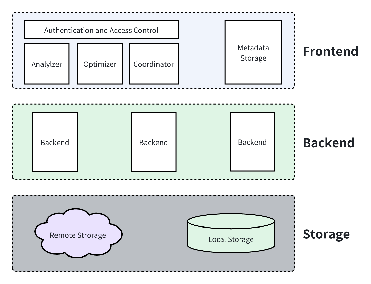
A Doris cluster consists of three components: Frontend (FE), Backend (BE), and Storage.

1. Frontend (FE): Primarily responsible for handling user requests, executing DDL and DML statements, optimizing tasks via the query optimizer, and aggregating execution results from Backends.
2. Backend (BE): Primarily responsible for query execution, processing data through a series of control logic and complex computations to return the data for users.
3. Storage: Managing data partitioning and data reads/writes. In Apache Doris, storage components are divided into local storage and remote storage.

3.2 Overview of Data Storage in Apache Doris

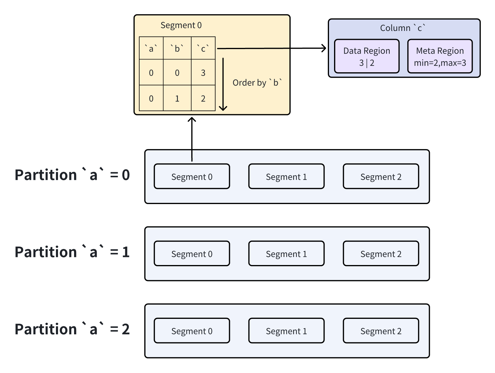
In Apache Doris’s data model, a table typically includes partition columns, Key columns, and data columns:

• At the storage layer, partition information is maintained in metadata. When a user query arrives, the Frontend can directly determine which partitions to read based on metadata.
• Key columns support data aggregation at the storage layer. In actual data files, Segments (split from partitions) are organized by the order of Key columns—meaning Key columns are sorted within each Segment.
• Within a Segment, each column is stored as an independent columnar data file (the smallest storage unit in Doris). These columnar files further maintain their own metadata (e.g., maximum and minimum values).

This content is only supported in a Feishu Docs

3.3 Overview of Data Pruning in Apache Doris

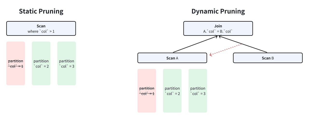
Based on when pruning occurs, data pruning in Apache Doris is categorized into two types: static pruning and dynamic pruning.

• Static pruning: Determined directly after the query SQL is processed by the parser and optimizer. It typically relies on pre-defined filter predicates in the SQL. For example, when querying data where a > 1, the optimizer can immediately exclude all partitions with a ≤ 1.
• Dynamic pruning: Determined during query execution. For example, in a query with a simple equivalent inner join, the Probe side only needs to read rows with values matching the Build side. This requires dynamically obtaining these values at runtime for pruning.

To elaborate on the implementation details of each pruning technique, we further classify them into four types based on pruning methods:

1. Predicate filtering (static pruning, determined by user SQL).
2. LIMIT pruning (dynamic pruning).
3. TopK pruning (dynamic pruning).
4. JOIN pruning (dynamic pruning).

The execution layer of an Apache Doris cluster usually includes multiple instances, and dynamic pruning requires coordination across instances. This increased the complexity of dynamic pruning. We will discuss the details later.

4. Predicate Filtering

In Apache Doris, static predicates are generated by the Frontend after processing by the Analyzer and Optimizer. Their effective timing varies based on the columns they act on:

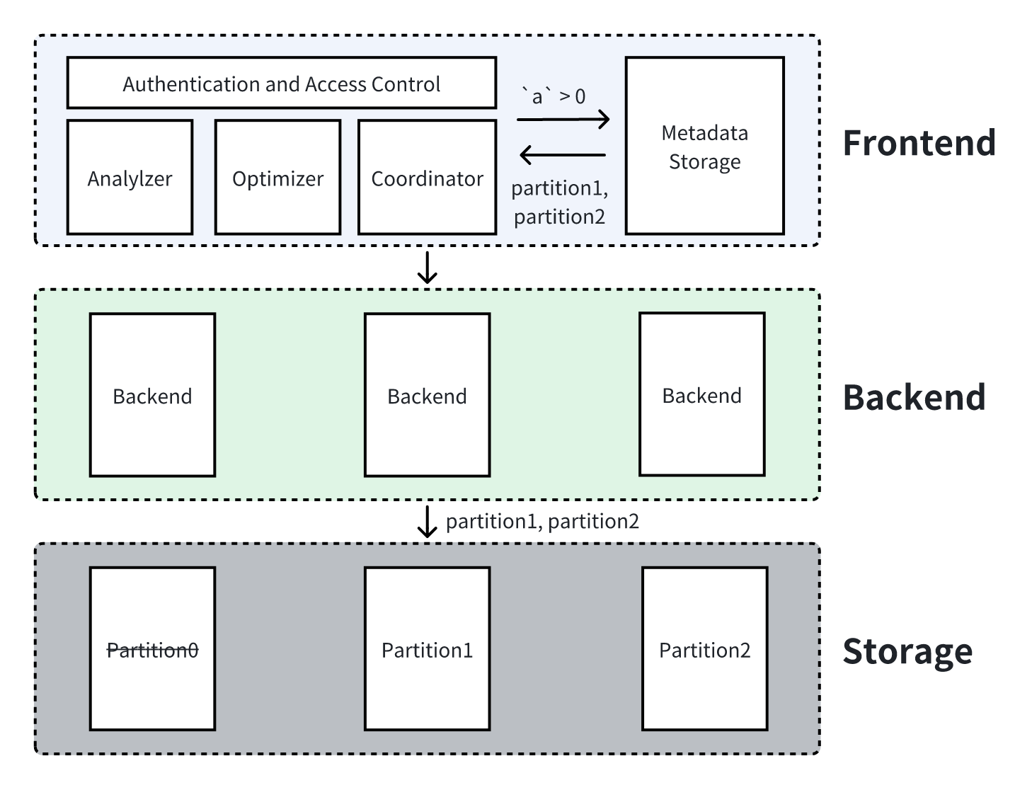
• Predicates on partition columns: The Frontend uses metadata to identify which partitions store the required data, enabling direct partition-level pruning (the most efficient form of data pruning).
• Predicates on Key columns: Since data is sorted by Key columns within Segments, we can generate upper and lower bounds for Key columns based on the predicates. Then, we use binary search to determine the range of rows to read.
• Predicates on regular data columns: First, we filter columnar files by comparing the predicate with metadata (e.g., max/min values) in each file. We then read all eligible columnar files and compute the predicate to get the row IDs of filtered data.

Example illustration: First, define the table structure:

CREATE TABLE IF NOT EXISTS `tbl` (
    a int,
    b int,
    c int
) ENGINE=OLAP
DUPLICATE KEY(a,b)
PARTITION BY RANGE(a) (
    PARTITION partition1 VALUES LESS THAN (1),
    PARTITION partition2 VALUES LESS THAN (2),
    PARTITION partition3 VALUES LESS THAN (3)
)
DISTRIBUTED BY HASH(b) BUCKETS 8
PROPERTIES (
    "replication_allocation" = "tag.location.default: 1"
);

Insert sample data to partition 1, partition 2, and partition 3:

| a | b | c | | ---- | ---- | ---- | | 0 | 0 | 1 | | 0 | 1 | 0 | | 1 | 0 | 3 | | 1 | 1 | 2 | | 2 | 0 | 5 | | 2 | 1 | 4 |

4.1 Predicate Filtering on Partition Columns

SELECT * FROM `tbl` WHERE `a` > 0;

As mentioned before, partition pruning is completed at the Frontend layer by interacting with metadata.

4.2 Predicate Filtering on Key Columns

Query (where b is a Key column):

SELECT * FROM `tbl` WHERE `b` > 0;

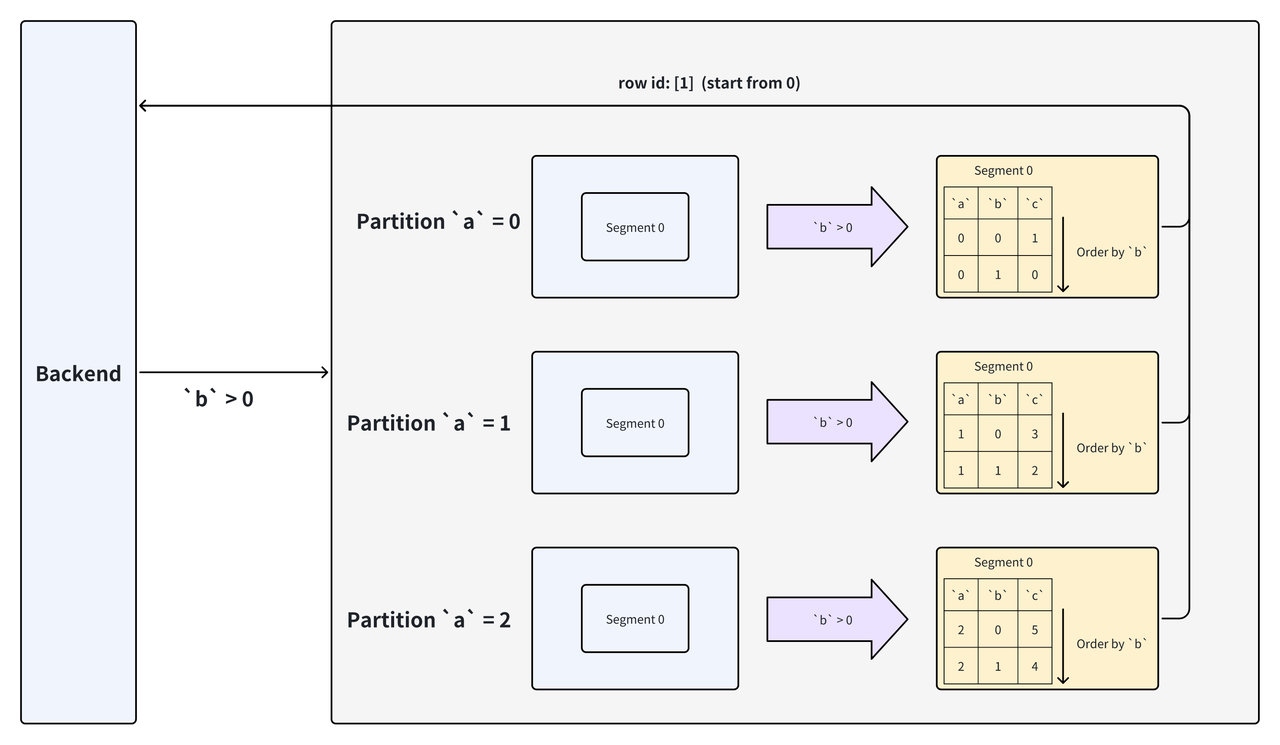
In this example, the storage layer uses the lower bound of the Key column predicate (0, exclusive) to perform a binary search on the Segment. It finally returns the row ID 1 (second row) of eligible data; the row ID is used to read data from other columns.

4.3 Predicate Filtering on Data Columns

Query (where c is a regular data column):

SELECT * FROM `tbl` WHERE `c` > 2;

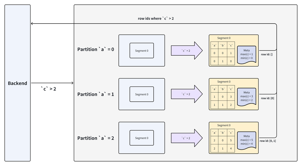
In this example, the storage layer utilizes data files from column c across all Segments for computation. Before computation, it skips files where the max value (from metadata) is less than the query’s lower bound (e.g., Column File 0 is skipped). For Column File 1, it computes the predicate to get matching row IDs, which are then used to read data from other columns.

5. LIMIT Pruning

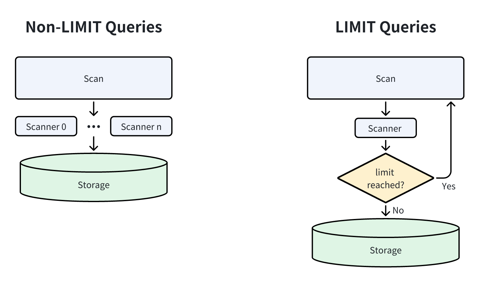
LIMIT queries are common in analytical tasks [11]. For regular queries, Doris uses concurrent reading to accelerate data scanning. For LIMIT queries, however, Doris adopts a different strategy to prune data early:

• LIMIT on Scan nodes: To avoid reading unnecessary data, Doris sets the scan concurrency to 1 and stops scanning once the number of returned rows reaches the LIMIT.
• LIMIT on other nodes: The Doris execution engine immediately stops reading data from all upstream nodes once the LIMIT is satisfied.

6. TopK Pruning

TopK queries are widely used in BI (Business Intelligence) scenarios. A TopK query retrieves the top-K results sorted by specific columns. Similar to LIMIT pruning, the naive approach—sorting all data and then selecting the top-K results, incurs high data scanning overhead. Thus, database systems typically use heap sorting for TopK queries. Optimizations during heap sorting (e.g., scanning only eligible data) can significantly improve query efficiency.

Standard Heap Sorting

The most intuitive method for TopK queries is to maintain a min-heap (for descending sorting). As data is scanned, it is inserted into the heap (triggering heap updates). Data not in the heap is discarded (no overhead for maintaining discarded data). After all data is scanned, the heap contains the required TopK results.

Theoretically Optimal Solution

The theoretically optimal solution refers to the minimum amount of data scanning needed to obtain correct TopK results:

• When the TopK query is sorted by Key columns: Since data within Segments is sorted by Key columns (see Section 3.2), we only need to read the first K rows of each Segment and then aggregate and sort these rows to get the final result.
• When the TopK query is sorted by non-Key columns: The optimal approach is to read and sort the sorted data of each Segment, and then select the required rows—avoiding scanning all data.

Doris includes targeted optimizations for TopK queries:

1. Local pruning: Scan threads first perform local pruning on data.
2. Global sorting: A global Coordinator aggregates and fully sorts the pruned data, then performs global pruning based on the sorted results.

Thus, TopK queries in Doris involve two phases:

• Phase 1: Read the sorted columns, perform local and global sorting, and obtain the row IDs of eligible data.
• Phase 2: Re-read all required columns using the row IDs from Phase 1 for the final result.

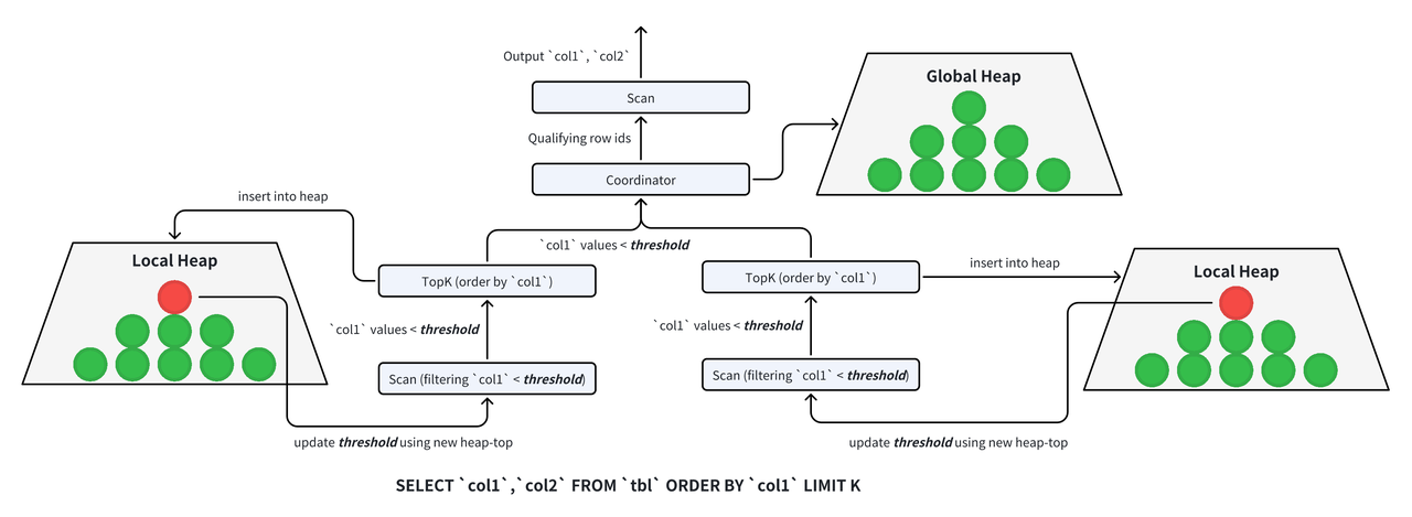
6.1 Local Data Pruning

During query execution:

1. Multiple independent threads read data.
2. Each thread processes the data locally.
3. Results are sent to an aggregation thread for the final result.

In TopK queries, each scan thread first performs local pruning:

• Each scan node is paired with a TopK node that maintains a heap of size K.
• If the number of scanned rows is less than K, scanning continues (insufficient data for TopK results).
• Once K rows are scanned, discard other unnecessary data. For subsequent scans, use the heap top element as a filter predicate (only scan data smaller than the heap top).
• This process repeats: scan data smaller than the current heap top, update the heap, and use the new heap top for filtering. This ensures only data eligible for TopK is scanned at each stage.

6.2 Global Data Pruning

After local pruning, N execution threads return at most N*K eligible rows. These rows require aggregation and sorting to get the final TopK results:

1. Use heap sorting to sort the N*K rows.
2. Output the K eligible rows and their row IDs to the Scan node.
3. The Scan node reads other columns required for the query using these row IDs.

6.3 TopK Pruning for Complex Queries

Local pruning does not involve multi-thread coordination and is straightforward (as long as the scan phase is aware of TopK, it can maintain and use the local heap). Global pruning is more complex: in a cluster, the behavior of the global Coordinator directly affects query performance.

Doris designs a general Coordinator applicable to all TopK queries. For example, in queries with multi-table joins:

• Phase 1: Read all columns required for joins and sorting, then perform sorting.
• Phase 2: Push the row IDs down to multiple tables for scanning.

7. JOIN Pruning

Multi-table joins are among the most time-consuming operations in database systems. From execution perspectives, less data means lower join overhead. A brute-force join (computing the Cartesian product) of two tables of size M and N has a time complexity of O(M*N). Thus, Hash Join is commonly used for higher efficiency:

1. Select the smaller table as the Build side and construct a hash table with its data.
2. Use the larger table as the Probe side to probe the hash table.

Ideally (ignoring memory access overhead and assuming efficient data structures), the time complexity of building the hash table and probing is O(1) per row, leading to an overall O(M+N) complexity for Hash Join. Since the Probe side is usually much larger than the Build side, reducing the Probe side’s data reading and computation is a critical challenge.

Apache Doris provides multiple methods for Probe-side pruning. Since the values of the Build-side data in the hash table are known, the pruning method can be selected based on the size of the Build-side data.

7.1 JOIN Pruning Algorithm

The goal of JOIN pruning is to reduce Probe-side overhead without compromising correctness. This requires balancing the overhead of constructing predicates from the hash table and the overhead of probing:

• Small Build-side data: Directly construct an exact predicate (e.g., an IN predicate). The IN predicate ensures all data used for probing is guaranteed to be part of the final output.

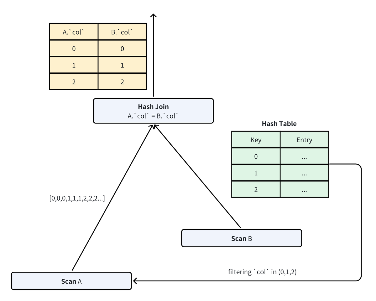
• Large Build-side data: Constructing an IN predicate incurs high deduplication overhead. For this case, Doris trades off some probing performance (reduced filtering rate) for a lower-overhead filter: Bloom Filter [5]. A Bloom Filter is an efficient filter with a configurable false positive probability (FPP). It maintains low predicate construction overhead even for large Build-side data. Since filtered data still undergoes join probing, correctness is guaranteed.

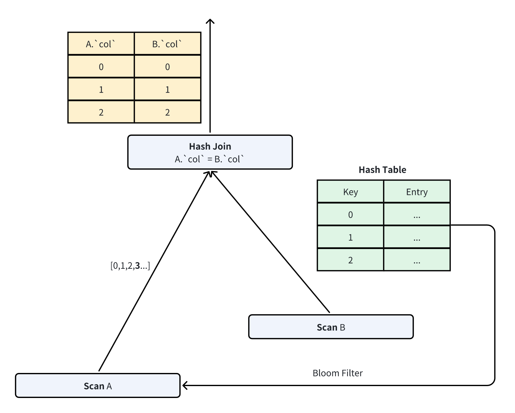
In Doris, join filter predicates are built dynamically at runtime and cannot be determined statically before execution. Thus, Doris uses an adaptive approach by default:

1. First, construct an IN predicate.
2. When the number of deduplicated values reaches a threshold, reconstruct a Bloom Filter as the join predicate.

7.2 JOIN Predicate Waiting Strategy

As Bloom Filter construction also incurs overhead, Doris’s adaptive pruning algorithm cannot fully avoid high query latency when the Build side has extremely high overhead. Thus, Doris introduces a JOIN predicate waiting strategy:

• By default, the predicate is assumed to be built within 1 second. The Probe side waits at most 1 second for the predicate from the Build side. If the predicate is not received, it starts scanning directly.
• If the Build-side predicate is completed during Probe-side scanning, it is immediately sent to the Probe side to filter subsequent data.

8. Conclusion and Future Work

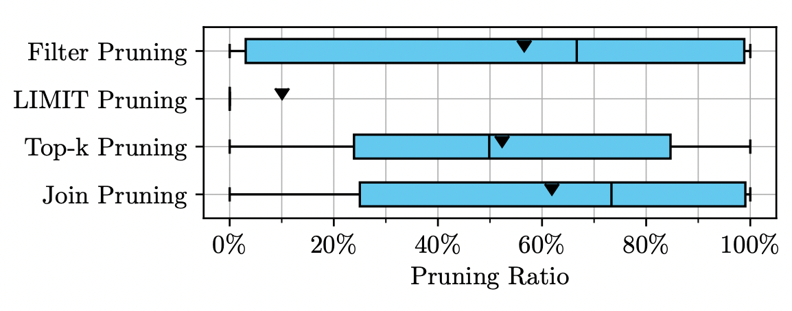
We present the implementation strategies of four data pruning techniques in Apache Doris: predicate filtering, LIMIT pruning, TopK pruning, and JOIN pruning. Currently, these efficient pruning strategies significantly improve data processing efficiency in Doris. According to the customer data from Snowflake in 2024 [12], the average pruning rates of predicate pruning, TopK pruning, and JOIN pruning exceed 50%, while the average pruning rate of LIMIT pruning is 10%. These figures demonstrate the significant impact of the four pruning strategies on customer query efficiency.

In the future, we will continue to explore more universal and efficient data pruning strategies. As data volumes grow, pruning efficiency will increasingly influence database system performance—making this a sustained area of development.

Reference

[1] Alexander van Renen and Viktor Leis. 2023. Cloud Analytics Benchmark. Proc. VLDB Endow. 16, 6 (2023), 1413–1425. doi:10.14778/3583140.3583156

[2] Alexander Hall, Olaf Bachmann, Robert Büssow, Silviu Ganceanu, and Marc Nunkesser. 2012. Processing a Trillion Cells per Mouse Click. Proc. VLDB Endow. 5, 11 (2012), 1436–1446. doi:10.14778/2350229.2350259

[3] Goetz Graefe. 2009. Fast Loads and Fast Queries. In Data Warehousing and Knowledge Discovery, 11th International Conference, DaWaK 2009, Linz, Austria, August 31 - September 2, 2009, Proceedings (Lecture Notes in Computer Science, Vol. 5691), Torben Bach Pedersen, Mukesh K. Mohania, and A Min Tjoa (Eds.). Springer, 111–124. doi:10.1007/978-3-642-03730-6_10

[4] Guido Moerkotte. 1998. Small Materialized Aggregates: A Light Weight Index Structure for Data Warehousing. In VLDB’98, Proceedings of 24rd International Conference on Very Large Data Bases, August 24-27, 1998, New York City, New York, USA, Ashish Gupta, Oded Shmueli, and Jennifer Widom (Eds.). Morgan Kaufmann, 476–487. http://www.vldb.org/conf/1998/p476.pdf

[5] Burton H. Bloom. 1970. Space/Time Trade-offs in Hash Coding with Allowable Errors. Commun. ACM 13, 7 (1970), 422–426. doi:10.1145/362686.362692

[6] Bin Fan, David G. Andersen, Michael Kaminsky, and Michael Mitzenmacher. 2014. Cuckoo Filter: Practically Better Than Bloom. In Proceedings of the 10th ACM International on Conference on emerging Networking Experiments and Technologies, CoNEXT 2014, Sydney, Australia, December 2-5, 2014, Aruna Seneviratne, Christophe Diot, Jim Kurose, Augustin Chaintreau, and Luigi Rizzo (Eds.). ACM, 75–88. doi:10.1145/2674005.2674994

[7] Martin Dietzfelbinger and Rasmus Pagh. 2008. Succinct Data Structures for Retrieval and Approximate Membership (Extended Abstract). In Automata, Languages and Programming, 35th International Colloquium, ICALP 2008, Reykjavik, Iceland, July 7-11, 2008, Proceedings, Part I: Tack A: Algorithms, Automata, Complexity, and Games (Lecture Notes in Computer Science, Vol. 5125), Luca Aceto, Ivan Damgård, Leslie Ann Goldberg, Magnús M. Halldórsson, Anna Ingólfsdóttir, and Igor Walukiewicz (Eds.). Springer, 385–396. doi:10.1007/978-3-540-70575-8_32

[8] Lothar F. Mackert and Guy M. Lohman. 1986. R* Optimizer Validation and Performance Evaluation for Local Queries. In Proceedings of the 1986 ACM SIGMOD International Conference on Management of Data, Washington, DC, USA, May 28-30, 1986, Carlo Zaniolo (Ed.). ACM Press, 84–95. doi:10.1145/16894.16863

[9] James K. Mullin. 1990. Optimal Semijoins for Distributed Database Systems. IEEE Trans. Software Eng. 16, 5 (1990), 558–560. doi:10.1109/32.52778

[10] https://doris.apache.org/

[11] Pat Hanrahan. 2012. Analytic database technologies for a new kind of user: the data enthusiast. In Proceedings of the ACM SIGMOD International Conference on Management of Data, SIGMOD 2012, Scottsdale, AZ, USA, May 20-24, 2012, K. Selçuk Candan, Yi Chen, Richard T. Snodgrass, Luis Gravano, and Ariel Fuxman (Eds.). ACM, 577–578. doi:10.1145/2213836.2213902

[12] Andreas Zimmerer, Damien Dam, Jan Kossmann, Juliane Waack, Ismail Oukid, Andreas Kipf. Pruning in Snowflake: Working Smarter, Not Harder. SIGMOD Conference Companion 2025: 757-770